Rebuilding ESP32-fluid-simulation: the advection and force steps of the sim task (Part 4)
If you’ve read Part 2 and Part 3 already, then you’re as equipped to read this part as I can make you. You would have already heard me mention that we should be passing in touch inputs, consisting of locations of velocities. You also would have already heard that we’re getting out color arrays. Some mechanism should be turning the former into the latter, and it should be broadly inspired by the physics, which is written out as partial differential equations. This post and the next post—the final ones—are about that mechanism. To be precise, this post covers everything but the pressure step, and the next will give that step its own airtime.
With that said, if I miss anything, the references I used might be helpful. That’s the GPU Gems chapter and Jamie Wong’s blog post, but there’s also Stam’s “Real-time Fluid Dynamics for Games” and “Stable Fluids”.
Now, to tell you what I’m going to tell you, a high-level overview is this:
- apply “semi-Lagrangian advection”, an implementation of the advection operator (for “advection”, see Part 3), to the velocities,
- apply the user’s input to the velocities,
- apply “divergence-free projection” to velocities in order to correct it (i.e. the pressure step briefed in Part 3 and to be explained in the next part) and finally,
- apply semi-Lagrangian advection to the density array with the updated velocities.
The process has four parts, and each part corresponds to a part of the physics. Let’s recall the partial differential equations that we ended up with in Part 3, that is:
\[\frac{\partial \rho}{\partial t} = - (\bold v \cdot \nabla) \rho\] \[\frac{\partial \bold v}{\partial t} = - (\bold v \cdot \nabla) \bold v - \frac{1}{\rho} \nabla p + \bold f\] \[\nabla \cdot \bold v = 0\]Setting aside the incompressibility constraint for now—that’s the third equation $\nabla \cdot \bold v = 0$—the equations can be split into four terms. That’s one term for each part of the process. To list them in the order of their corresponding steps, there’s the advection of the velocity $-(\bold v \cdot \nabla) \bold v$, the applied force $\bold f$, the pressure $- \frac{1}{\rho} \nabla p$, and the advection of the density $-(\bold v \cdot \nabla) \rho$.
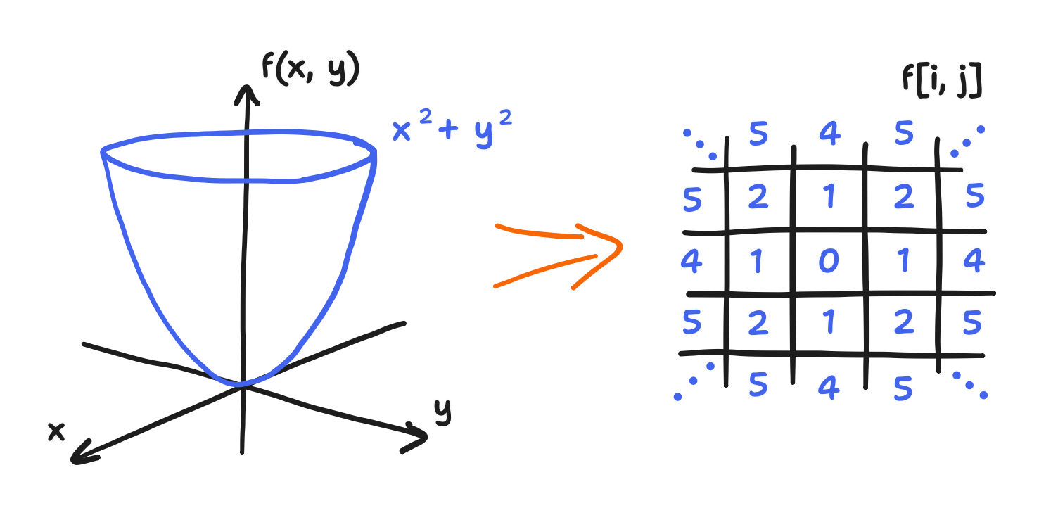
Before we get into each term and its corresponding part of the process, there’s a key piece of context to keep in mind. We’re faced with the definitions of $\frac{\partial \rho}{\partial t}$ and $\frac{\partial \bold v}{\partial t}$ here, and they have solutions which are density and velocity fields that evolve over time. That’s not computable. Computers can’t operate on fields—the functions of continuous space that they are—much less operate on ones that continuously vary over time. Instead, time and space need to be “discretized”.
Let’s tackle the discretization of time first. Continuous time can be approximated by a sequence of closely-spaced points in time. Usually, those points in time are regularly spaced apart by a timestep $\Delta t$, In other words, we use the sequence $\{\; 0,\; \Delta t,\; 2 \Delta t,\; 3 \Delta t,\; \dots \;\}$. The result should be that a field at some time $t$ in the sequence can be approximately expressed in terms of the field at the previous time $t_0 - \Delta t$. That is, we should be able to calculate an update to the fields. You may see how this is useful for running simulations. This general idea is called “numerical integration”, the simplest case being Euler’s method—yes, that Euler’s method, if you still remember it. In other cases, methods like implicit Euler, Runge-Kutta, and leapfrog integration offer better accuracy and/or stability, but that’s out-of-scope.
Now, let’s tackle the discretization of space. Continuous space can be approximated by a mesh of points, each point being associated with the value of the field there. In the simplest case, that mesh is a regular grid. Also remember that fields are functions of location. Combining these two things, we get the incredibly convenient conclusion that discretized fields can be expressed as an array of values. For each index into the array $(i, j)$, there is a corresponding point on the grid $(x_i, y_j)$, and for every point, there is a value of the field at that point. If we wanted to initialize an array from some known field, we could just evaluate the field on each point of the grid and then assign the value to the associated cell of the array.
Side note: it’s a fair question to ask here why $(i, j)$ doesn’t correspond to—say—$(x_j, y_i)$ instead. Why does $i$ select the horizontal component and not the vertical one? This continues from my tangent about indexing in Part 2. The answer is that you could go about it that way and then derive a different but entirely consistent discretization. In fact, I originally had it that way. However, I switched out of that to keep all the expressions looking like how they do in the literature. So, in short, the reason is just convention.
Second side note: this is not to say that the array is a matrix. The array is only two-dimensional because the space is two-dimensional. If the space was three-dimensional, then so would be the array. And forget about arrays if the mesh isn’t a grid! So, most matrix operations wouldn’t mean anything either. It’d be more correct to think of discretized fields as very long vectors, but we’re encroaching on a next-post matter now.
A grid discretization is what Stam went with, and for that reason, it’s what’s used here.
A key result of discretizing space is that the differential operators can be approximated by differences (i.e. subtraction) between the values of the field at a point and its neighbors. In particular, using a grid can make the partial derivatives into something incredibly simple: $\frac{\partial}{\partial x}$ into the value of the right neighbor minus the value of the left neighbor and $\frac{\partial}{\partial y}$ into the top minus the bottom. But that’s getting into “finite difference methods”, of which the pressure step is one such method. We’ll get to that in the next post. For now, it’s enough to say that, in general, discretizing with a grid is the simple choice for making computers operate on fields.
With that said, we’ll soon see that “semi-Lagrangian advection” does something unique with the grid.
To sum up this “just for context” moment, to compute an approximate solution to the presented partial differential equations, we need two levels of discretization. First, we need to discretize time, turning it into a scheme of updating the density and velocity fields repeatedly. Then, we need to discretize space to make the update computable. And so, time is replaced with a sequence, and space is replaced with a grid. All this is because computers cannot handle functions of continuous time nor functions of continuous space, let alone functions of both like an evolving field. Now, all this is quite abstract, and that’s because each part invokes the discretization of time and space slightly differently, and we’ll go into the details of each.
With all that said, in the face of our definitions of $\frac{\partial \rho}{\partial t}$ and $\frac{\partial \bold v}{\partial t}$, this generally means that the density/concentration field (which I’m currently just calling the density field out of expediency) and the velocity field become just density and velocity arrays, and we should be able to calculate their updates. In this situation, we can update the arrays in accordance with the partial differential equations by going term by term, hence why each step of the overall process corresponds to a single term. (Though, I’m not sure if the implicit assumption of independence between the terms that underlies going term by term is just an expedient approximation or our math-given right. Anyway…) Let’s go over the four parts, step by step.
The first step is the “semi-Lagrangian advection” of the velocities, implementing the $-(\bold v \cdot \nabla) \bold v$ term. A key highlight here: Stam’s treatment of the advection term is not a finite difference method, yet it still uses discretization with a grid! I’d also like to highlight a bit of how Stam arrived at this method. All that information is largely documented between “Stable Fluids” and “Real-Time Fluid Dynamics for Games”.
In “Stable Fluids”, there is a formal analysis that involves a technique called a “method of characteristics”. It’s a whole proof, but a sketch of it is this: at every point $\bold x$ (that’s the coordinate vector $\bold x$, as covered in Part 2), there is a particle, and that particle arrived there from somewhere. Let $\bold{p}(\bold x, t)$ be its path, such that the current location is defined by the equality $\bold{p}(\bold x, t_0) = \bold x$ where $t_0$ is the current time. Then, $\bold{p}(\bold x, t_0 - \Delta t)$ is where the particle was in the previous time.
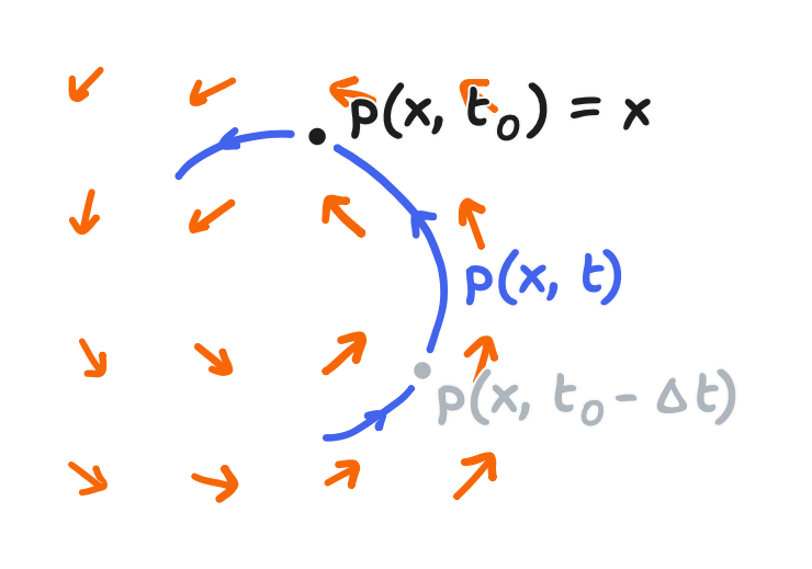
As a result, the particle must have carried its properties along the way, and one of them is said to be momentum, or in other words, velocity. Therefore, an advection update looks like the assignment of the field value at the previous location, $\bold{p}(\bold x, t_0 - \Delta t)$, to the field at the current location, $\bold x$. This is the result of Stam’s analysis, and it can be written as the following:
\[\bold{v}_\text{advect}(\bold x) = \bold{v}(\bold{p}(\bold x, t_0 - \Delta t))\]There is a unique time discretization here, but we’re not done yet! It’s still not computable because it’s missing a discretization of space. Of course, Stam presented one in “Stable Fluids” too. The calculation of $\bold{v}_\text{advect}$ can be done at just the points on the grid, and for each point, a “Runge-Kutta back-tracing” on the velocity field can be used to find $\bold{p}(\bold x, t_0 - \Delta t)$.
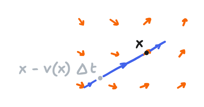
I won’t get into how that works, and I won’t have to in a moment. We’re one further approximation away from the method that appears in “Real-time Fluid Dynamics for Games” (and also the GPU Gems article and Wong’s post). Quite simply, if finding the path from $\bold{p}(\bold x, t_0 - \Delta t)$ to $\bold x$ can be called a “nonlinear” backtracing, then it’s replaced with a linear backtracing. The path is approximated with a straight line that extends from $\bold x$ in the direction of the velocity there:
\[\bold{v}_\text{advect}(x) = \bold{v}(\bold x - \bold{v}(\bold x) \Delta t, t)\]or in other words $\bold x - \bold{v}(\bold x) \Delta t$ replaces $\bold{p}(\bold x, t - \Delta t)$
This expression is usually shown on its own, but it’s really three parts: a “method of characteristics” analysis that comprises a time discretization, a space discretization using a grid, and a further approximation using a linear backtracing.
Anyway, the found point almost certainly doesn’t coincide with a point on the grid, so Stam dealt with this by “bilinearly interpolating” between the four closest velocity values.
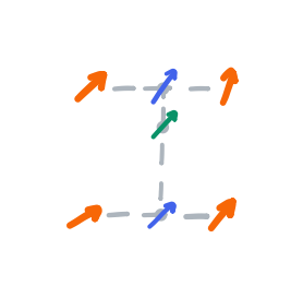
For more information on that, see the above link to Wikipedia. It’s got a better explanation of bilinear interpolation than one I can make—diagrams included. With that said, bilinear interpolation also amounts to very little code.
template<typename T>
using TPromoted = decltype(std::declval<T>() * std::declval<float>());

template <class T>
static TPromoted<T> lerp(float di, T p1, T p2)
{
    return p1 * (1 - di) + p2 * di;
}

template <class T>
static TPromoted<T> billinear_interpolate(float di, float dj, T p11, T p12,
                                          T p21, T p22)
{
    return lerp(di, lerp(dj, p11, p12), lerp(dj, p21, p22));
}
For this project, which in C++, that code uses templates. That lets it handle multiple types, which it will see because—remember—there are two advection terms! There’s one for velocity and there’s one for density. Much of the work presented for velocity will be reused, via templates. And if you’re wondering about the using TPromoted expression. The simplest way to write linear interpolation is with floating-point, and once we’re in floating point, we may as well stay in floating point, only converting back at the very end. This includes floating-point vector classes, which is why decltype is used instead of just a float type.
With that in mind, it’s simply a matter of computing the source and getting the bilinear interpolation with that point. Here’s a sample of code from the project that does this.
template <class T>
static T sample(T *p, float i, float j, int dim_x, int dim_y, bool no_slip) {
    bool x_under = i < 0;
    bool x_over = i >= dim_x - 1;
    bool y_under = j < 0;
    bool y_over = j >= dim_y - 1;

    bool x_oob = x_under || x_over;
    bool y_oob = y_under || y_over;

    float i_floor = floorf(i), j_floor = floorf(j);
    float di = i - i_floor, dj = j - j_floor;
    int ij;

    if (!x_oob && !y_oob) {   // typical case: not near the boundary
        ij = index(i_floor, j_floor, dim_x);
        return billinear_interpolate(di, dj, p[ij], p[ij + dim_x], p[ij + 1],
                                     p[ij + dim_x + 1]);
    }

    // OMITTED
}

template <class T, class U>
void advect(T *next_p, T *p, Vector2<U> *vel, int dim_x, int dim_y, float dt,
            bool no_slip)
{
    for (int i = 0; i < dim_x; i++) {
        for (int j = 0; j < dim_y; j++) {
            int ij = index(i, j, dim_x);
            Vector2<float> source = Vector2<float>(i, j) - vel[ij] * dt;
            next_p[ij] = sample(p, source.x, source.y, dim_x, dim_y, no_slip);
        }
    }
}
Here, the advect function loops over every point on the grid, calculating the source for each and assigning the result of the sample function. The sample function in turn calls the earlier given bilinear_interpolate function.
But I’ve omitted the rest of the sample function! Notice that it returns early if the source is not near the boundary. That creates a fast path, and that means the omitted code was for handling when it is near the boundary.
So, what have I hidden? I’ll answer with another question. What if the backtracing sends us to the boundary of the domain, or even beyond it?
It’s a fair question to ask, and it’s an important question because what we should do here directly depends on what the boundary is physically. In our case, the boundary is a solid wall. Here, I turn to the GPU Gems article, where it’s written that the “no-slip” condition hence applies, which just means the velocity there must be zero. Why the change again in my references? The “Stable Fluids” paper assumed a different physical condition, “periodic” boundaries that essentially imply a tile-able cell or a “toroidal” i.e. donut-shaped domain, but the “Real-time Fluid Dynamics for Games” paper chose a somewhat looser condition that was still based on solid walls. Between that and no-slip conditions, no-slip conditions are easier to build upon. For starters, a no-slip condition is more easily implemented inside a bilinear interpolation scheme—inside the sample function, that is.
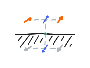
For now, let’s focus on the bottom row. Below the bottom row, we can construct a ghost row that always takes the negative of its values. Therefore, any linear interpolation at the halfway point between the bottom row and the ghost row must be equal to zero. That is, the halfway line between them achieves the no-slip condition, thereby simulating the solid wall. From there, if the backtracing gives a position that is beyond the halfway line, it should just be clamped to it. Finally, this approach with the ghost row extends to all sides of the domain.
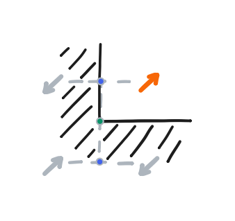
We also need to define the value of the ghost corner formed by a ghost row and ghost column. I didn’t see a rigorous treatment of them in my references, and I’ve seen that the corners might not matter much in practice. Still, the “no-slip” condition has a nice internal consistency that just gives us this definition. At the intersection of the halfway lines, the velocity there must also be zero. From this, we can form an equation involving the value of the ghost corner, and its solution is that the ghost corner should take on the value of the real corner—not its negative! Rather, it can be thought of as the ghost row taking the negative of the value at the end of the ghost column, which is itself a negative, and so making a double negative.
That said, the project doesn’t actually handle the boundary with ghost rows/columns, which is how it’s done in “Real-time Fluid Dynamics for Games” and the GPU Gems article. It used to, but now it uses something different but equivalent. To understand the difference, it is important to recognize that the negative values are just constructs on the way to defining the halfway line, where the no-slip condition is enforced and beyond which no source point is supposed to exist.
Let’s now draw the bilinear interpolation as a 3D surface. The construction of the halfway line ends up looking like this.
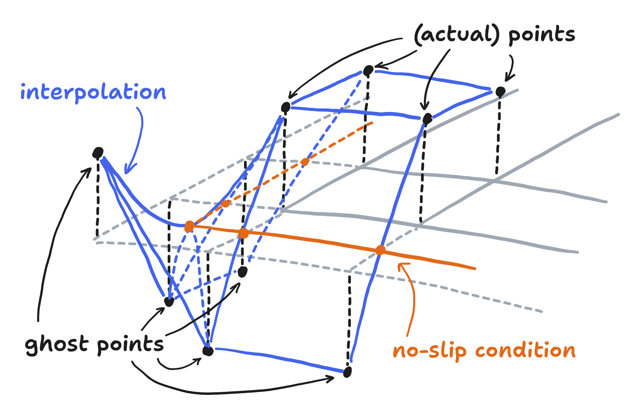
The ghost rows and columns take on negative values, and so the surface does indeed flip in sign as it crosses the halfway line. As mentioned before though, source points are to never cross that line, and they’re to be clamped to it if they do. As a result, the samples of that surface will never flip in sign. In that sense, the negative values are just virtual—being part of the construction but not having its own impact.
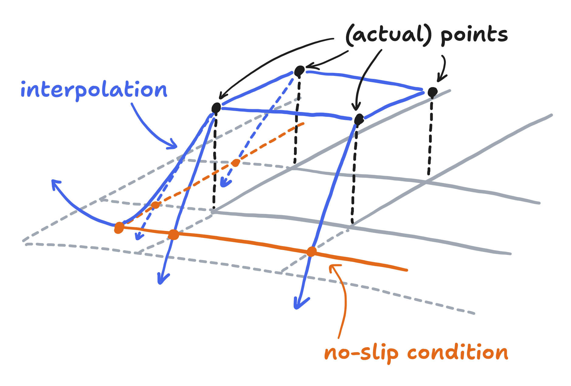
It follows that, so long as the halfway line is constructed another way, the ghost rows and columns can be done away with entirely. The project does this by computing an “overshoot factor” that reduces the velocity to zero as the “overshoot” approaches 0.5, i.e. the halfway line. If it exceeds 0.5, then it too can be clamped so that the surface samples still never flip sign.
As a surface, it looks like this.
And here’s its code—the rest of the sample function.
template <class T>
static T sample(T *p, float i, float j, int dim_x, int dim_y, bool no_slip) {
    // OMITTED

    // interpolate along the boundary
    T p_edge;
    if (x_oob && y_oob) {  // on a corner
        ij = index((x_under? 0 : dim_x - 1), (y_under? 0 : dim_y - 1), dim_x);
        p_edge = p[ij];
    } else if (x_oob) {  // on left or right boundary
        ij = index((x_under? 0 : dim_x - 1), j_floor, dim_x);
        p_edge = lerp(dj, p[ij], p[ij + dim_x]);
    } else {  // y_oob, on bottom or top boundary
        ij = index(i_floor, (y_under? 0 : dim_y - 1), dim_x);
        p_edge = lerp(di, p[ij], p[ij + 1]);
    }

    if (!no_slip) {
        return p_edge;
    }

    // apply discount to implement no-slip, with zero at the boundary and beyond
    float overshoot_factor = 1.0f;
    if (x_oob) {
        float overshoot_x = x_under ? -i : i - (dim_x - 1);
        overshoot_factor *= overshoot_x < 0.5 ? (1 - 2 * overshoot_x) : 0;
    }
    if (y_oob) {
        float overshoot_y = y_under ? -j : j - (dim_y - 1);
        overshoot_factor *= overshoot_y < 0.5 ? (1 - 2 * overshoot_y) : 0;
    }
    return overshoot_factor * p_edge;
}
It’s worth noticing here that applying the overshoot factor is skipped if no_slip is false. That is the case for advecting things besides velocity, where reducing the value to zero at the boundary just isn’t physical. For example, false is passed for the density.
Altogether, we had a “method of characteristics” update that was discretized with a grid, linear backtracing, and bilinear interpolation, with boundaries being handled so that a no-slip condition is enforced. It’s enforced by constructing halfway lines where the velocity is made to be zero, be that by creating ghost rows and columns with negative values or by reducing the value by an overshoot factor. All this implements advection, one of the components of a fluid simulation, as demonstrated by it being a term in the differential equation.
An important comment about all of this: according to Stam, the “method of characteristics” update, before discretization, is “unconditionally stable” because no value in $\bold{v}_\text{advect}$ can be larger than the largest value in $\bold v$ because $\bold{v}_\text{advect}$ always is some value in $\bold v$. From there, his discretization with bilinear interpolation preserved the stability because $\bold{v}_\text{advect}$ is always between some values in $\bold v$ (or zero, if the boundary is involved).
In the past, I had written fluid simulations that didn’t have unconditional stability, and they all blew up unless I took small timesteps. Getting to take large timesteps here—not needing to do loop after loop just to cover a span of time equal the blink of an eye—is critical to running this sim on an ESP32.
And now, here’s some more general conclusions.
- In “Real-time Fluid Dynamics for Games”, Stam goes on to state that “the idea of tracing back and interpolating” is a kind of “semi-Lagrangian method”. Doing linear backtracing, as opposed to something else like the aforementioned Runge-Kutta method, isn’t quintessential to that classification. It remains a useful approximation, though.
- The key feature of this method is the unconditional stability that comes from the interpolation not exceeding the original values, and that’s a useful constraint to carry forward. For example, if the simulation blows up, something wasn’t done correctly.
- Generally speaking, this advection method isn’t the end-all and be-all of advection methods, and the field of fluid simulation is much larger than that. And it escapes me—go look to other sources for those.
Moving on from the semi-Lagrangian advection of velocity (and density), the second step is to apply the user’s input to the velocity array. This corresponds to the $\bold f$ term, the external forces term. This isn’t something Stam had set in stone, since what makes up the external forces really depends on the physical situation being simulated. In our case, we want someone swirling their arm in the water, and so external forces must be derived from the touch data. That’s the touch data we had the touch task generate in Part 2, and here’s where it comes into play.
Recall that a touch input consists of a position and a velocity. Let $\bold{x}_i$ and $\bold{v}_i$ be the position and velocity of the $i$-th input in the queue. Naturally, we should want to influence the velocities around $\bold{x}_i$ in the direction of $\bold{v}_i$. Under this general guidance, I could have gone about it in the way that was done in the GPU Gems article. That was to add a “Gaussian splat” to the velocity array, and that “splat” was formally expressed as something like this
\[\bold{f}_i \, \Delta t \, e^{\left\Vert \bold{x} - \bold{x}_i \right\Vert^2 / r^2}\]where $\bold{f}_i$ is a vector with some reasonably predetermined magnitude but with a direction equal to that of $\bold{v}_i$. From the multiplication $\bold{f}_i \Delta t$, you may notice that the time discretization in play is just Euler’s method and that the space discretization in play is to just evaluate it at the points of the grid. Across all the inputs in the queue, the update would have been
\[\bold{v}_\text{force}(\bold{x}) = \bold{v}(\bold{x}) + \sum_{i = 0}^N \bold{f}_i \, \Delta t \, e^{\left\Vert \bold{x} - \bold{x}_i \right\Vert^2 / r^2}\]where $N$ is the number of items in the queue. I had two issues with it. First, I specifically wanted to capture how you can’t push the fluid immediately around your arm faster than the speed of your arm (though the offshoot vortices are free to spin faster). This was especially important when someone was moving the stylus very gently. Second, evaluating the splat at every single point would’ve been expensive. My crude solution to this was to just set $\bold{v}(\bold{x}_i)$ to be equal to $\bold{v}_i$. In code, that turns out to merely be the following
struct drag msg;
while (xQueueReceive(drag_queue, &msg, 0) == pdTRUE) {
    int ij = index(msg.coords.y, msg.coords.x, N_ROWS);
    Vector2<float> swapped(msg.velocity.y, msg.velocity.x);
    velocity_field[ij] = swapped;
}
where, if you’re confused about the apparent “axes swap”, see the section in Part 2, I can write this code as
\[\bold{v}_\text{force}(\bold{x}_i) = \bold{v}_i\] \[\bold{v}_\text{force}(\bold{x}) = \bold{v}(\bold{x}) \text{ for } \bold{x} \not= \bold{x}_i \text{ for any } i\]The third step is the pressure step, corresponding to the $- \frac{1}{\rho} \nabla p$ term. Out of all the terms in the definition of $\frac{\partial \bold v}{\partial t}$, it must be calculated last, capping off the velocity update before we can proceed to the density update. I already discussed this in Part 2, but in short, the pressure does not represent a real process here. Rather, it is a correction term that eliminates divergence in the velocity field. This ensures the incompressibility constraint, $\nabla \cdot \bold v = 0$. (Technically, the specific formulation that Stam presents doesn’t eliminate it entirely, but it does eliminate most of it. We can get into that in the next part.) Since it’s not a real process, no time discretization is in play. Rather, the updated velocity field is straight-up not valid until the correction is applied.
It would be more correct to state that Stam’s fluid simulation follows the modified definition that he presents in “Stable Fluids”, that is
\[\frac{\partial \bold v}{\partial t} = \mathbb{P} \big( - (\bold v \cdot \nabla) \bold v + \nu \nabla^2 \bold v + \bold f \big)\]where $\mathbb{P}$ is a linear projection onto the space of velocity fields with zero divergence. This definition clearly shows that $\mathbb{P}$ must be calculated last, though it hides the fact that calculating it does involve a gradient. Anyway, applying the reductions that we’ve been running with so far, that would just be
\[\frac{\partial \bold v}{\partial t} = \mathbb{P} \big( - (\bold v \cdot \nabla) \bold v + \bold f \big)\]where, we’ve again set $\nu$ to zero.
This happens to be the pressure projection that is shown in the GPU Gems chapter. That said, to keep the notation simple, I won’t continue to use it. And on the matter of actually calculating it, there’s so much to say in the next part. I’ll provide the code then as well.
That just leaves the fourth and final step, the semi-Lagrangian advection of the density, corresponding to the term $-(\bold v \cdot \nabla) \rho$. Well, that’s the only term in the definition of $\frac{\partial \rho}{\partial t}$, and we already covered it when we covered the velocity advection! There are no more obstacles here. The only thing I’d mention is that extending the fluid sim to full color is quite trivial. Instead of advecting a single density field, we can advect three independent density fields—one for red dye, one for blue dye, and one for green dye—or equivalently a vector field of densities. The project happens to go with the latter approach.
That fills most of the outline, implementing every part of the reduced Navier-Stokes equations except for the pressure step. That’s the applied force and the semi-Lagrangian advection of the velocity and density. There, we paid special attention to the derivation and the no-slip boundary condition, since that comes from the physical situation being simulated. We also went a bit into the general idea of discretizing time (i.e. numerical integration) and discretizing space. That’s everything I know about those steps that I think could help their implementation. In the next and final post, we’ll go over what, exactly, the pressure step is, including the relevant linear algebra. Stay tuned!