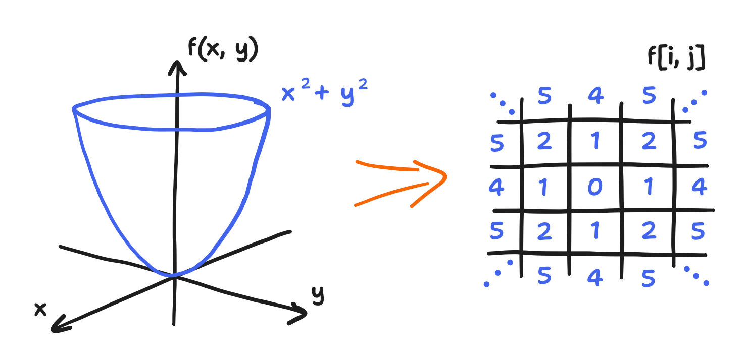
<?xml version="1.0" encoding="utf-8"?><feed xmlns="http://www.w3.org/2005/Atom" ><generator uri="https://jekyllrb.com/" version="3.10.0">Jekyll</generator><link href="http://kennypeng.com/feed.xml" rel="self" type="application/atom+xml" /><link href="http://kennypeng.com/" rel="alternate" type="text/html" /><updated>2026-03-01T22:13:23+00:00</updated><id>http://kennypeng.com/feed.xml</id><title type="html">just for context by Kenny Peng</title><subtitle>A blog about my personal projects  and the rich backgrounds they rely on
</subtitle><author><name>Kenny Peng</name><email>kenny@kennypeng.com</email></author><entry><title type="html">Rebuilding ESP32-fluid-simulation: the pressure projection step of the sim task (Part 5)</title><link href="http://kennypeng.com/2024/09/26/esp32_fluid_sim_5.html" rel="alternate" type="text/html" title="Rebuilding ESP32-fluid-simulation: the pressure projection step of the sim task (Part 5)" /><published>2024-09-26T00:00:00+00:00</published><updated>2024-09-26T00:00:00+00:00</updated><id>http://kennypeng.com/2024/09/26/esp32_fluid_sim_5</id><content type="html" xml:base="http://kennypeng.com/2024/09/26/esp32_fluid_sim_5.html"><![CDATA[<p>It’s been a while since my last post, but let’s bring this series to its finale. Out of all the parts of the fluid sim, the last piece I have not explained is the pressure projection. The code alone doesn’t reveal the great deal of context that goes into its design. Here’s a hint: it’s actually a linear algebra routine involving a “sparse matrix”. Though it’s possible these days to implement the pressure projection without needing to know all that context, thanks to articles like <a href="https://jamie-wong.com/2016/08/05/webgl-fluid-simulation/">Jamie Wong’s post</a>, <a href="https://developer.nvidia.com/gpugems/gpugems/part-vi-beyond-triangles/chapter-38-fast-fluid-dynamics-simulation-gpu">the GPU Gems chapter</a>, and Stam’s <a href="https://www.dgp.toronto.edu/~stam/reality/Research/pdf/GDC03.pdf">“Real-Time Fluid Dynamics for Games”</a>, achieving a believable fluid simulation on an ESP32 <em>would have been impossible</em>. I’ve personally tried it before, and after knowing? All I needed was to switch in a technically superior method. There was a reason why I dedicated airtime to this—let me explain.</p>

<p>In <a href="/2023/09/22/esp32_fluid_sim_3.html">part 3</a>, we covered the Navier-Stokes equations, and in <a href="/2024/01/20/esp32_fluid_sim_4.html">part 4</a>, we covered how parts of the equations were discretized differently. Well, to begin with I need to cover one last thing that involves continuous fields and not discrete arrays: the “Helmholtz-Hodge decomposition”.</p>

<p>It’s mentioned in the GPU Gems chapter, and for that Stam’s 1999 “Stable Fluids” paper is cited. In the end, I had found “Stable Fluids” to be the definitive place to start looking for context, and there I borrow much of my understanding. Now, it itself cites a section of the book <em>A mathematical introduction to fluid mechanics</em> by Chorin and Marsden. Building upon this section, I’ll get into what the “Helmholtz-Hodge decomposition” is. Though, I won’t get into why it is i.e. all of the book preceding that section. That’s outside the scope I want to take here, but that’s also outside what I can comfortably do—I’ll admit. With that said, what is it, and how do we apply it?</p>

<p>We can derive the pressure projection from the decomposition. To begin, the decomposition itself is this: given some vector field $\bold{w}$ that is defined over a bounded space, it can be taken as the following sum</p>

\[\bold{w} = \bold{v} + \nabla p\]

<p>where $\nabla p$ is the gradient of a scalar field and $\bold v$ is a vector field that has zero divergence everywhere in the space and zero flow across its boundary. In other words, every vector field can be broken down into two components, one with all of its original divergence and one with zero divergence, and the former is <em>necessarily</em> the gradient of some scalar field. In part 3, I mentioned that a linear projection $\mathbb{P}$ is applied to the velocity field in order to make it valid, and remember that “valid” means that it satisfies the incompressibility constraint by having zero divergence. A definition for that linear projection can be built upon the Helmholtz-Hodge decomposition.</p>

<p>Let $\bold w$ be the uncorrected velocity field. Since we want its zero-divergence component, we need to isolate $\bold{v}$. That gives us this expression.</p>

\[\bold{v} = \bold{w} - \nabla p\]

<p>However, before we can subtract $\nabla p$ from $\bold w$, we need to find what $p$ is in the first place! The Helmholtz-Hodge decomposition tells us that such a $p$ exists, but the problem is that it does not tell us <em>how</em> to find it. Therein lies the meat of the pressure projection. In this context, $p$ is not just some scalar field; $p$ stands for “pressure”.</p>

<p>Also in the Chorin and Marsden section, you’d find that the proof of the Helmholtz-Hodge decomposition builds upon the pressure being the solution to a particular <a href="https://en.wikipedia.org/wiki/Boundary_value_problem">“boundary value problem”</a>, one that Stam noted to involve a case of <a href="https://en.wikipedia.org/wiki/Poisson%27s_equation">“Poisson’s equation”</a>. In a “boundary value problem”, we’re given a bounded space as a domain, the governing differential equations that a function on that space (i.e. a field) must satisfy, and the values that the function (and/or values of that function’s derivative) must take on the boundary i.e. the “boundary conditions”.</p>

<figure>
<img src="/images/2024-09-26/figure1.png" alt="A bounded region, and the inside is colored blue with hatch fill and labeled with Poisson's equation whereas the boundary is labeled with another equation and covered in arrows, pointing outward and in various lengths" />
<figcaption>

The three principal parts of a boundary value problem: a bounded domain, a governing equation, and the boundary condition(s).

</figcaption>
</figure>

<p>Regarding “Poisson’s equation”, I’m not qualified to opine about it or anything, so I’ll just say that it’s a partial differential equation where one scalar field is equal to the Laplacian of another scalar field. If there’s an intuitive meaning to it, that’s currently lost on me.</p>

<p>
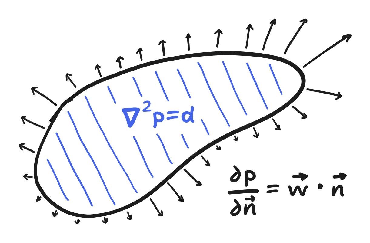
Anyway, the boundary value problem is this: given $\bold{w}$, $p$ should satisfy the following case of Poisson’s equation</p>

\[\nabla^2 p = \nabla \cdot \bold{w}\]

<p>on the domain, whereas on the boundary its <a href="https://en.wikipedia.org/wiki/Directional_derivative">“directional derivative”</a> is specified.</p>

<p>
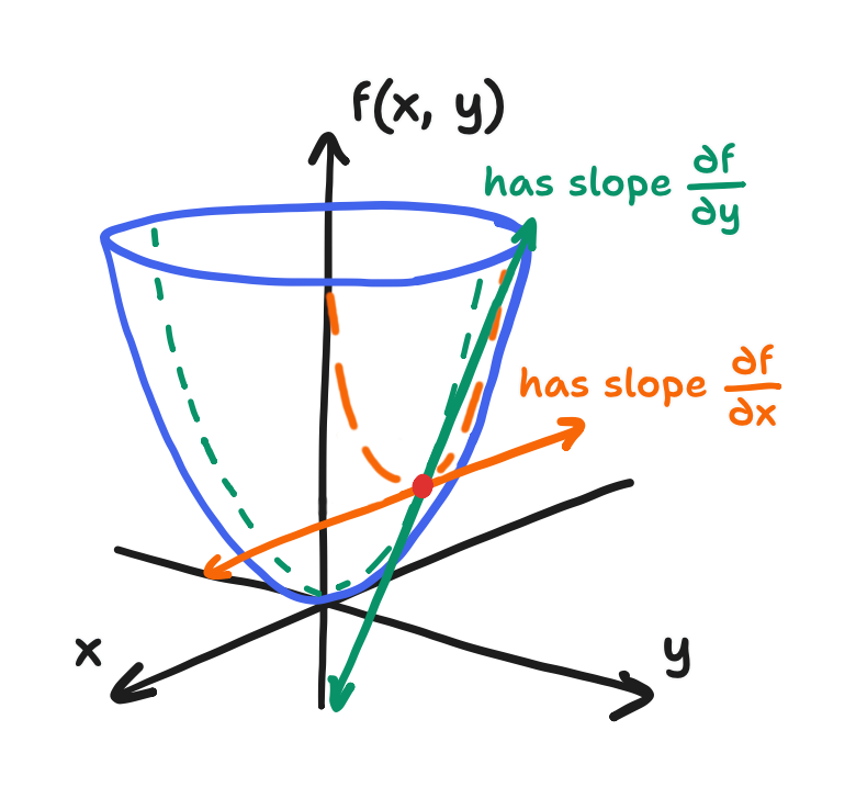
When I say “directional derivative”, I’d like you to recall that explanation of the partial derivative I did in Part 3, where I mentioned that $\frac{\partial p}{\partial x}$ and $\frac{\partial p}{\partial y}$ were just the slopes of two lines in the many that make up the plane tangent to the field. The “directional derivative” is the slope of a potentially different line, the one running in the direction that the derivative is being taken with respect to. (This definition also goes to show that the typical partials $\frac{\partial p}{\partial x}$ and $\frac{\partial p}{\partial y}$ are special cases of the directional derivative, being taken in the $+x$- and $+y$-directions.)</p>

<figure>
<img src="/images/2024-09-26/figure2.png" alt="A three-dimensional plot of x, y, and a function of x and y and a line tangent to the surface, annotated with a dashed line running from the point of intersection to the x-y plane, where lies a small arrow labelled n and point the in-plane direction in which the tangent line runs" />
</figure>

<p>
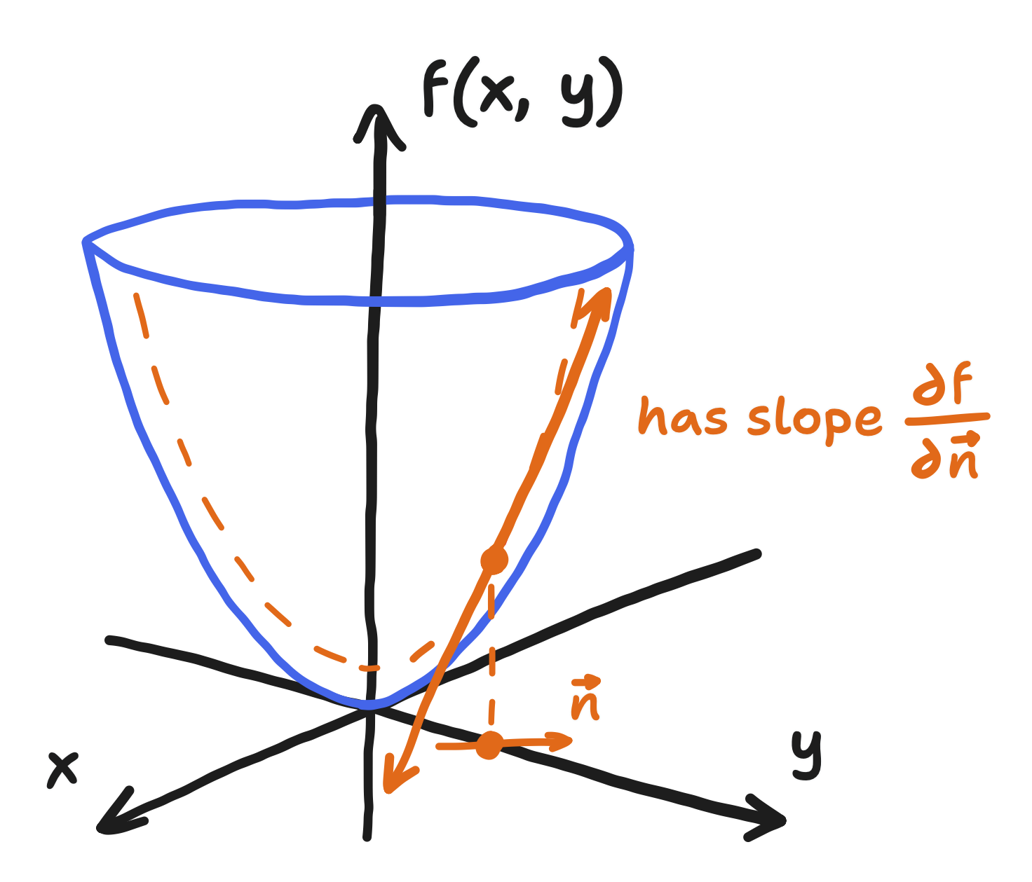
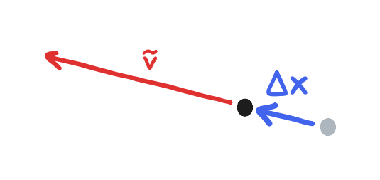
It is often denoted as $\frac{\partial f}{\partial \bold{v}}$, where $\bold{v}$ is a vector that points in the direction that the field $f$ is being taken with respect to. Furthermore, it is defined as the dot product between the gradient $\nabla f$ and $\tilde{\bold{v}}$, where $\tilde{\bold{v}}$ is the unit vector in that direction.</p>

\[\frac{\partial f}{\partial \bold{v}} \equiv \tilde{\bold{v}} \cdot \nabla f\]

<p>In this case, the directional derivative with respect to the normal (the direction perpendicular to the boundary and pointing outwards) is equal to the component of $\bold{w}$ that is in that direction. A specification of the derivative, not the value, of $p$ like this is said to be a “Neumann” boundary condition. Formally, the boundary condition is written like this:</p>

\[\frac{\partial p}{\partial \bold{n}} = \bold{w} \cdot \bold{n} \enspace \text{on} \enspace \partial D\]

<figure>
<img src="/images/2024-09-26/figure3.png" alt="Three arrows running outward from a point on a 2D surface: one labelled w and pointed in some direction, one labelled n and pointed in the direction perpendicular to the surface, and one labelled w dot n and pointed in the same direction as n" />
</figure>

<p>
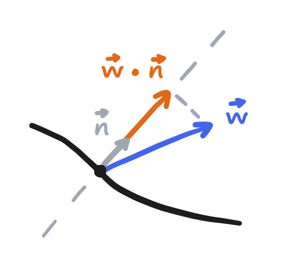
So, our boundary value problem involves a case of Poisson’s equation and Neumann boundary conditions, not to mention the domain, which should be representative of the screen, i.e. a rectangle. There are many ways to solve this, but we’ll start by again turning to discretization with a grid. This time, though, it’ll be an entire finite difference method.</p>

<div class="info-panel">

  <h3 id="review-the-finite-difference-discretization">Review: The finite difference discretization</h3>

  <p>I mentioned them in passing in Part 4, but you may or may not be familiar with the “finite difference” approximation of a derivative. A “finite difference” can be taken quite literally: it’s the “difference” (i.e. subtraction) between the values of a function at points separated by a “finite” (i.e. not infinitesimal) distance. It’s what happens when you <em>don’t</em> take the limit inside the definition of the derivative.</p>

\[\frac{df}{dx} = \lim_{h \to \infty} \frac{f(x) - f(x-h)}{h} \approx \frac{f(x) - f(x-\Delta x)}{\Delta x}\]

  <figure> 
<img src="/images/2024-09-26/figure4.png" alt="A plot of a function of x as a curve with a point in the center, three other points preceding it but increasing in proximity, lines going through each and the center point, and a tangent line through the center point" />
<figcaption>

A function, a center $x$, a tangent line there, and secant lines going through it and some other points of decreasing $\Delta x$. Notice how the slope gets closer to the slope of the tangent as $\Delta x$ decreases.

</figcaption>
</figure>

  <p>
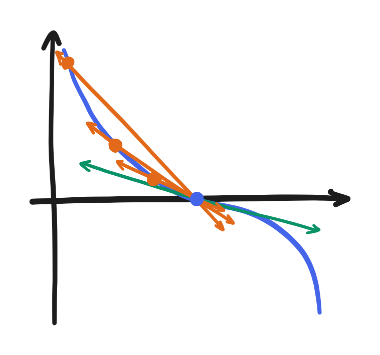
In general, there are many different ways to approximate the derivative using different pairs (or even larger combinations of) of neighboring points. Anyway, that’s out of scope. We should focus on the common cases. The above expression shows the “backward” difference, taking a point and its preceding point. The other two common cases are the “forward” difference and the “central” difference, which come from different, yet equivalent, definitions of the derivative.</p>

  <p>The forward difference uses a point and its succeeding point,</p>

\[\frac{df}{dx} \approx \frac{f(x + \Delta x) - f(x)}{\Delta x}\]

  <figure> 
<img src="/images/2024-09-26/figure5.png" alt="A plot of a function of x as a curve with a point in the center, three other points succeeding it but increasing in proximity, lines going through each and the center point, and a tangent line through the center point" />
<figcaption>

Notice how this also works when approaching from the other direction.

</figcaption>
</figure>

  <p>
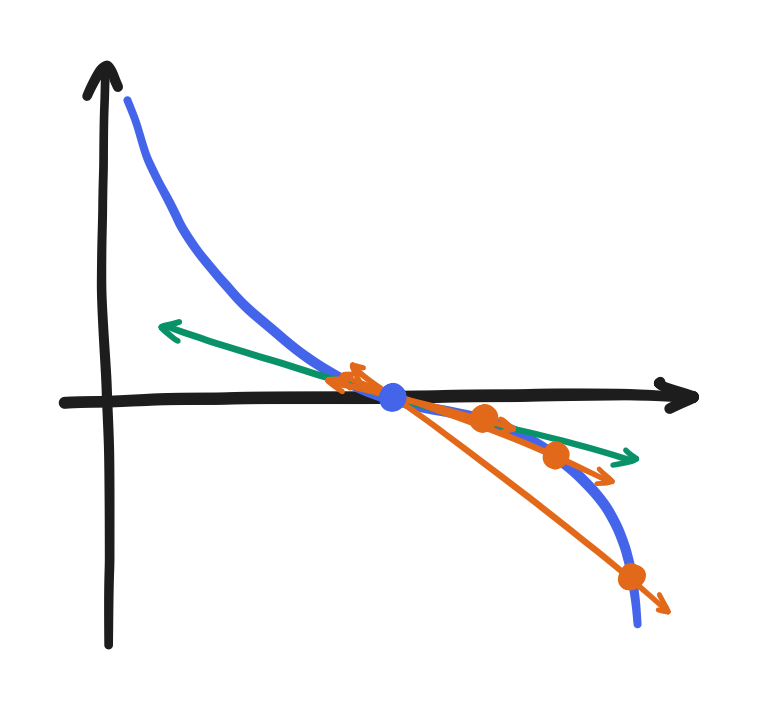
and the central difference uses the preceding point and the succeeding point.</p>

\[\frac{df}{dx} \approx \frac{f(x + \Delta x) - f(x - \Delta x)}{2 \Delta x}\]

  <figure> 
<img src="/images/2024-09-26/figure6.png" alt="A plot of a function of x as a curve with a point in the center, three points preceding it but increasing in proximity, three points succeeding it but increasing in proximity, lines each going through a preceding point and its corresponding succeeding point, and a tangent line through the center point" />
<figcaption>

Notice how this also works when drawing a line through a preceding point and a succeeding point, approaching from each side.

</figcaption>
</figure>

  <p>
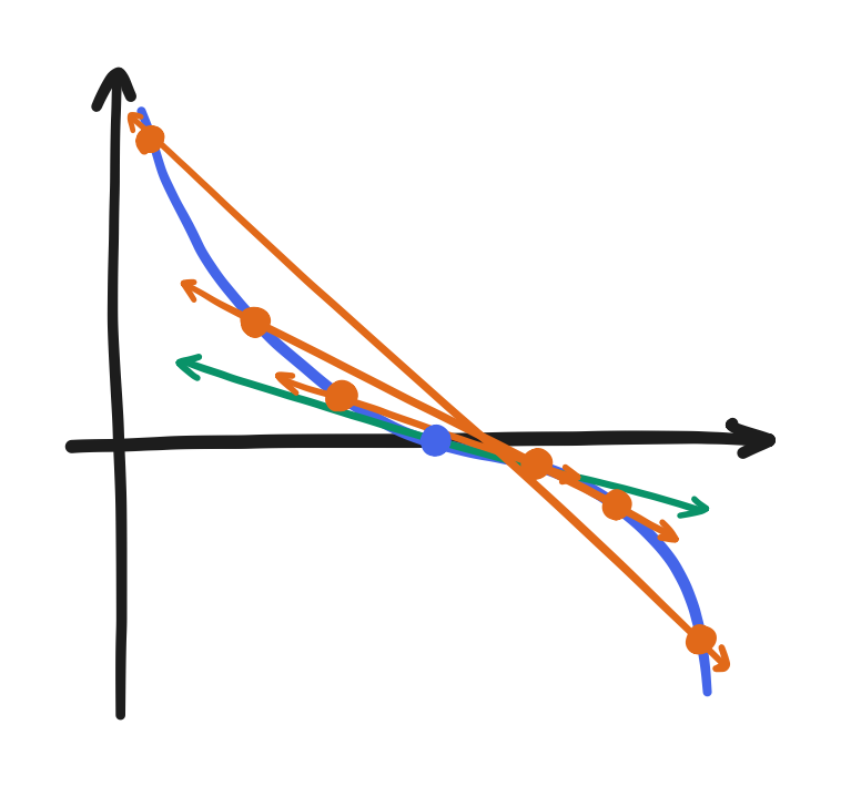
All of these expressions converge on the same value as $\Delta x$ shrinks, but we’ll end up using the central difference the most. That said, the forward and backward differences also get involved in today’s scheme.</p>

  <p>Anyway, because we discretized the fields with grids, this approximation is useful to us. First, extending this idea to partial derivatives is quite simple! Recall that it’s the derivative of a field with respect to one component while keeping all others constant. Because we discretized space with a grid, all points have left, right, top, and bottom neighbors (all besides the ones on the boundary, but we’ll get to them at some point). So, we can use the preceding and succeeding neighbors in each direction, $\frac{\partial f}{\partial x}$ using the left and right and $\frac{\partial f}{\partial y}$ using the top and bottom.</p>

\[\frac{\partial f}{\partial x} \approx \frac{f(x + \Delta x, y) - f(x - \Delta x, y)}{2 \Delta x}\]

\[\frac{\partial f}{\partial y} \approx \frac{f(x, y + \Delta y) - f(x, y - \Delta y)}{2 \Delta y}\]

  <figure> 
<img src="/images/2024-09-26/figure7.png" alt="Amid a grid of points (colored grey), five points are connected in a structure involving a center point and its top, bottom, left, and right neighbors labeled plus delta y, minus delta y, minus delta x, and plus delta x respectively" />
<figcaption>

The <a href="https://en.wikipedia.org/wiki/Five-point_stencil">five-point stencil</a>, showing all the points involved in our finite difference discretization

</figcaption>
</figure>

  <p>
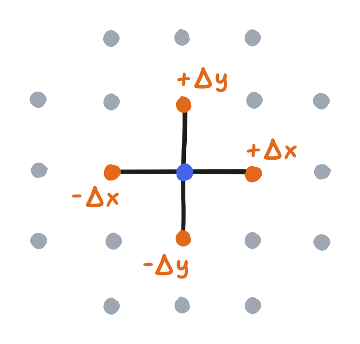
Finally, recall that a field that’s discretized with a grid can be represented by an array, and so we can rewrite the above central differences using indices.</p>

\[g_x[i, j] = \frac{f[i+1, j] - f[i-1, j]}{2 \Delta x}\]

\[g_y[i, j] = \frac{f[i, j+1] - f[i, j-1]}{2 \Delta y}\]

  <p>With this, approximating the differential operators is as easy as taking their definitions and replacing each partial derivative with its finite difference counterpart. Let’s write out the ones we’ll use for the rest of this article.</p>

  <p>Discretizing the gradient and the divergence with the central differences gets the following:</p>

\[\nabla f = \begin{bmatrix} \displaystyle \frac{\partial f}{\partial x} \\[1em] \displaystyle \frac{\partial f}{\partial y} \end{bmatrix} \approx \begin{bmatrix} \displaystyle \frac{f[i+1, j] - f[i-1, j]}{2 \Delta x} \\[1em] \displaystyle \frac{f[i, j+1] - f[i, j-1]}{2 \Delta y} \end{bmatrix}\]

\[\nabla \cdot \bold{f} = \frac{\partial f_x}{\partial x} + \frac{\partial f_y}{\partial y} \approx \frac{f[i+1, j] - f[i-1, j]}{2 \Delta x} + \frac{f[i, j+1] - f[i, j-1]}{2 \Delta y}\]

  <p>That leaves the Laplacian. There happens to be a “but actually” to discuss here. You may recall from Part 3 that the Laplacian is the divergence of the gradient but also that it can be written as a sum of the second partial (non-mixed) derivatives.</p>

\[\nabla^2 f \equiv \nabla \cdot (\nabla f) = \frac{\partial^2 \! f}{\partial x^2} + \frac{\partial^2 \! f}{\partial y^2}\]

  <p>One possible discrete approximation—one that uses what we’ve already mentioned—is to take the discrete gradient <em>and then</em> take the discrete divergence. Instead, the typical thing to do builds upon the <em>latter</em> definition. A second derivative can itself be approximated with finite differences, and the central difference way to do it is this:</p>

\[\frac{d^2 \! f}{d x^2} \approx \frac{f(x+\Delta x) - 2f(x) + f(x - \Delta x)}{\Delta x^2}\]

  <p>After extending this approximation to the partial derivative and rewriting it in terms of array values, that latter definition becomes the following.</p>

\[\frac{\partial^2 \! f}{\partial x^2} + \frac{\partial^2 \! f}{\partial y^2} \approx \frac{f[i+1, j] - 2 f[i,j] + f[i-1, j]}{\Delta x^2} + \frac{f[i, j+1] - 2 f[i, j] + f[i, j-1]}{\Delta y^2}\]

  <p>Finally, if the grid is square—that is, $\Delta x = \Delta y$—then the $f[i,j]$ terms can be combined cleanly, and it just reduces to this:</p>

\[\frac{\partial^2 \! f}{\partial x^2} + \frac{\partial^2 \! f}{\partial y^2} \approx \frac{f[i+1,j] + f[i-1,j] + f[i, j+1] + f[i, j-1] - 4 f[i, j]}{\Delta x^2}\]

  <p>This is how the Laplacian is typically discretized, but it’s actually <em>not</em> equal to the discrete divergence of the discrete gradient. Going about it that way happens to get you the above but with $\Delta x$ and $\Delta y$ being twice as large and the neighbor’s neighbor being used (two to the left, two to the right, etc.). And, for the record, it didn’t look that good when I tried it.</p>

  <p>Really, it goes to show that the “Stable Fluids” discretization will be simple but not very faithful to the original boundary value problem. Once before, years ago, I didn’t realize it could be flawed, and I lost many hours because of that. On another note, I reached out a year ago to Stam about it, and he mentioned that he instead used the “marker-and-cell (MAC) method” in his past professional work on Maya (now Autodesk Maya) and I managed to work out after that the MAC method <em>does</em> happen to make the two equal.</p>

  <p>Anyway, that’s the finite difference discretization (or, well, a simple case of it) and how it is applied to the gradient, divergence, and Laplacian. It’s a fundamental concept to grasp because—as you will see—a discrete approximation of differential operators can turn our boundary value problem into something we can solve.</p>

</div>

<p>So, how do we use finite differences to solve the problem? At this point, the “Stable Fluids” paper goes on to use a technique that will not fly here. If you’re curious about it, Stam had originally defined a different problem that used periodic boundary conditions, i.e. wrap-around from right to left, top to bottom, etc., and that allowed him to use the fast Fourier Transform (FFT). Since we’d want the fluid to collide into and generally stay within the boundary, we’re stuck with Neumann boundary conditions and no FFT. Anyway, we can instead turn to the method found in Stam’s “Real-time Fluid Dynamics for Games” or also the GPU Gems chapter. Those sources essentially line up with “Stable Fluids” up to here. But first, I’ll take the time to emphasize some of the context.</p>

<p>To begin with, we need to apply the finite difference discretization to the boundary value problem. I’ll say here that we need to treat <em>both</em> the governing equation and the boundary conditions <em>simultaneously</em>.</p>

<p>The governing equation, being just a case of Poisson’s equation, is simple enough; we just replace the Laplacian and the divergence with their discrete counterparts. In those articles, the central difference version with a square grid is used, so that’s what we’ll use here. Overall, the governing equation becomes this:</p>

\[\frac{p[i+1, j] + p[i-1, j] + p[i, j+1] + p[i, j-1] - 4 p[i, j]}{\Delta x^2} = d[i, j]\]

<p>where $d[i, j]$ is defined as the discrete divergence of $\bold{w}$</p>

\[d[i,j] = \frac{w_x[i+1, j] + w_x[i-1, j] + w_y[i, j+1] + w_y[i, j-1]}{2 \Delta x}\]

<p>Notice here that $d[i, j]$ is purely a function of some elements of $\bold{w}$, which is the given uncorrected velocity. That means we can treat $d[i, j]$ as a known value. Also notice here that discretizing the Poisson equation causes us to not have a just one unknown anymore. Given some $i$ and $j$, there are <em>five</em> unknown elements of $p$ and one known element of $d$, and that’s not solvable.</p>

<p>
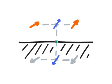
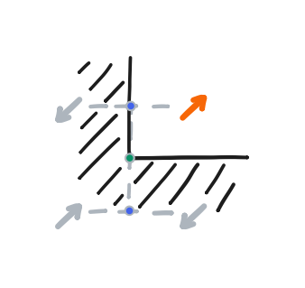
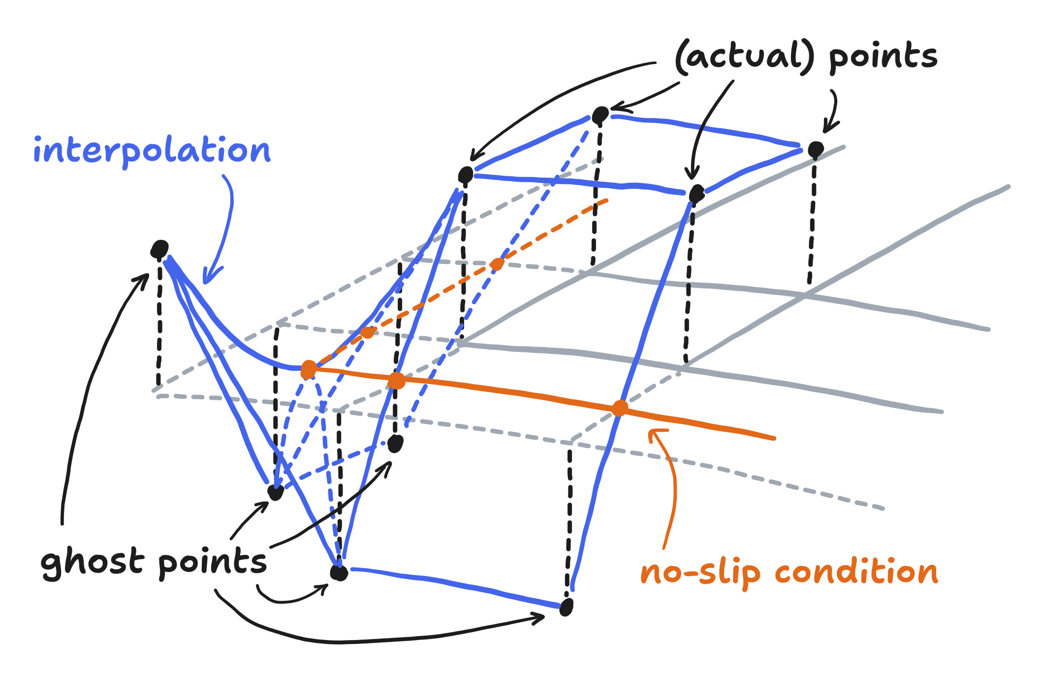
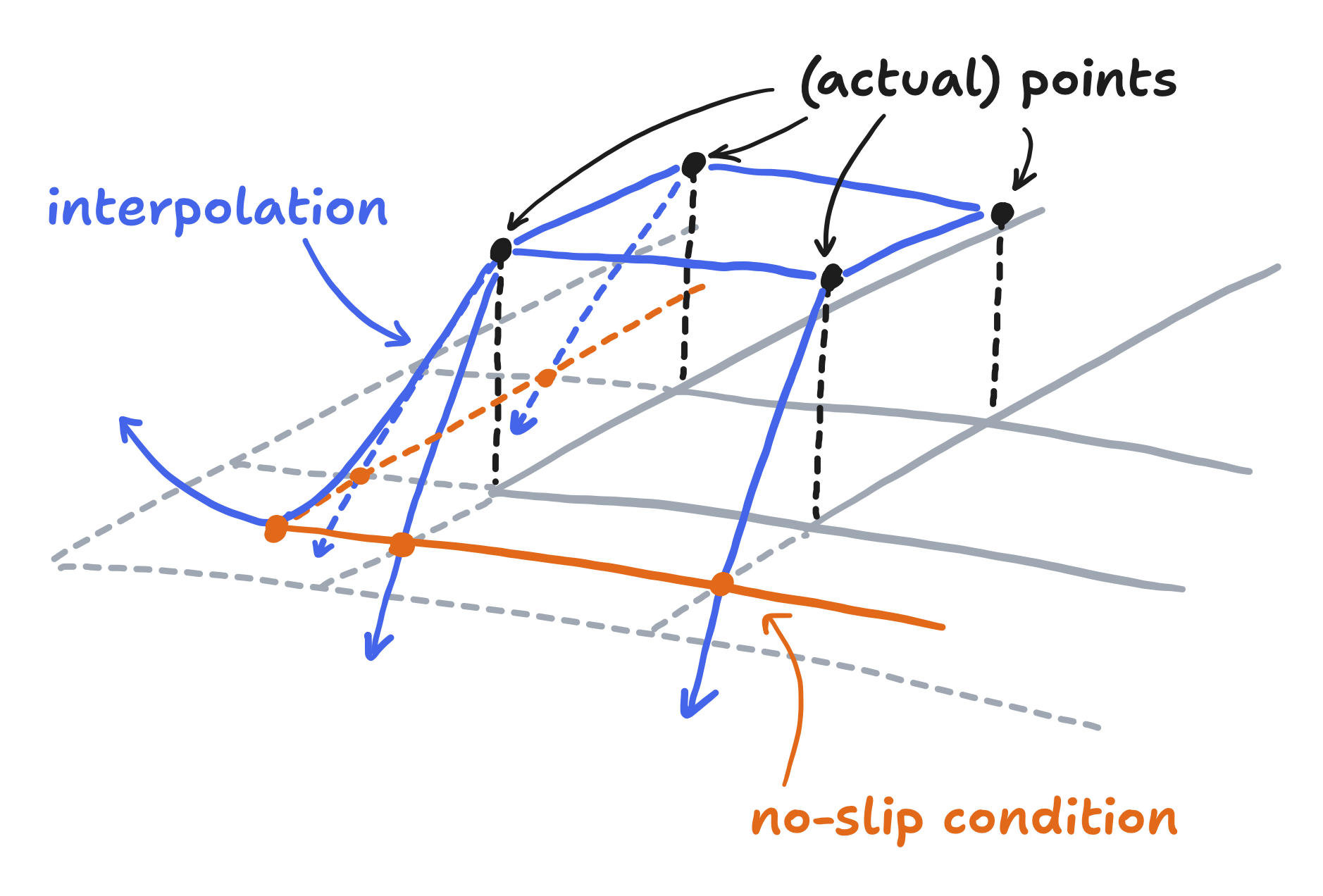
Before we deal with that, the boundary conditions are the other half we need to discretize. You may have noticed a plot hole here already: there isn’t always a left, up, right, or down neighbor. $p[i-1, j]$ doesn’t exist if $i = 0$. Now, remember how we used ghost points to complete the bilinear interpolation at the boundary? I’ll show that we can discretize our Neumann condition with the same ghost points that we covered in part 4, and in doing so we’ll find out what to do here.</p>

<p>I do have to preface this with something real quick, though. As I brought up earlier, the directional derivative of $p$ with respect to the normal is equal to the component of $\bold w$ in that direction. This statement I pulled from the Chorin and Marsden book. However, in Stam’s “Stable Fluids” and the GPU Gems article, the same boundary value problem is presented but with the directional derivative stated as being equal to <em>zero</em>. It’s a clear discrepancy.</p>

<p>It comes from grid choice. Remember from Part 4 that the boundary is supposed to simulate a wall that runs <em>between</em> the last real row and the ghost row. That was accomplished by making the ghost rows and columns take the negative because that makes the value of the bilinear interpolation at the “wall” equal to zero by definition. If $\bold{w}$ at the boundary is zero, then $\bold{w} \cdot \bold{n}$ must be zero. If $\bold{w} \cdot \bold{n}$ is zero, then even when following the definition from Chorin and Marsden, $\frac{\partial p}{\partial \bold{n}}$ must be zero.</p>

<p>That out of the way, our boundary condition just manifests as setting $\frac{\partial p}{\partial x}$ or $\frac{\partial p}{\partial y}$ because the domain is rectangular. Let’s see what to do on the top side first. There, the normal direction is the $+y$-direction. That is, $\frac{\partial p}{\partial \bold{n}} = 0$ manifests as $\frac{\partial p}{\partial y} = 0$. We then replace $\frac{\partial p}{\partial y}$ with its finite difference counterpart, but there’s a twist. The forward difference, not the central difference, is used. That gets us the following.</p>

\[\frac{p[i, N] - p[i, N-1]}{\Delta x} = 0\]

<p>where $i$ is any horizontal index, $N-1$ is the vertical index of the last real row, and $N$ is the vertical index of the ghost row. The implication of this statement is obvious: the ghost row must take on values equal to that of the real row.</p>

\[p[i, N] = p[i, N-1]\]

<div class="note-panel">

  <p>Though it may sound strange that we switched from applying the central difference to the forward difference, I think we can imagine together what it would imply if we kept it: at the top boundary, the central difference must be equal to zero</p>

\[\frac{p[i, N] - p[i, N-2]}{2 \Delta x} = 0\]

  <p>and therefore the ghost row should take on the values of the <em>second-to-last</em> row.</p>

\[p[i, N] = p[i, N-2]\]

  <p>That conclusion doesn’t sound as natural.</p>

</div>

<p>The same conclusion should be expected for all sides. For the bottom side, it’s reached by applying the backward difference on $\frac{\partial p}{\partial y} = 0$. For the right side, the forward difference on $\frac{\partial p}{\partial x} = 0$, and for the left, the backward difference on $\frac{\partial p}{\partial x} = 0$. It should sound quite similar to what we did for the bilinear interpolation, though back then the ghost row had to take on the negative.</p>

<p>To recap, the governing equation is discretized with finite differences, and the Neumann boundary condition is handled by reintroducing the ghost row but this time letting it essentially be the real row repeated (same going for the columns). That completes the finite difference version of our boundary value problem! Which leaves solving it, and with what else but a computer? Now, there’s that, and then there’s solving it with an ESP32 for the computer. If my goal was to explain the former, then quoting my sources would’ve been effective enough, but here’s comes the necessary context.</p>

<p>For one, didn’t I say this involved “sparse matrices”? Here they are.</p>

<div class="info-panel">

  <h3 id="review-sparse-matrices">Review: Sparse matrices</h3>

  <p>You may or may not be familiar with <a href="https://en.wikipedia.org/wiki/Sparse_matrix">“sparse matrices”</a>. If you are, then you would know that they enable a great deal of optimization on a computer—to a point where even the big-O complexity is lower—without changing <em>any</em> of the linear algebra stuff. With such drastic improvement for free on the table, “sparse matrices” are an essential topic. And that’s all for, well, “sparse matrices” just being matrices with a lot of zeroes.</p>

  <figure> 
<img src="/images/2024-09-26/figure8.png" alt="A black-and-white image consisting of white squares and black squares, revealing a diagonal component plus speckle" />
<figcaption>

An image created by taking the elements of a sparse, symmetric matrix (not the ones we'll soon see, but some other one) and filling the zero elements with white and the nonzero elements with black. By <a href="https://commons.wikimedia.org/wiki/File:Finite_element_sparse_matrix.png">Oleg Alexandrov via Wikimedia Commons</a>, where it was released into the public domain.

</figcaption>
</figure>

  <p>Generally speaking, zero can be effectively implemented by doing nothing or storing nothing. Conversely, actual computation and memory is focused on the non-zero elements.</p>

</div>

<p>
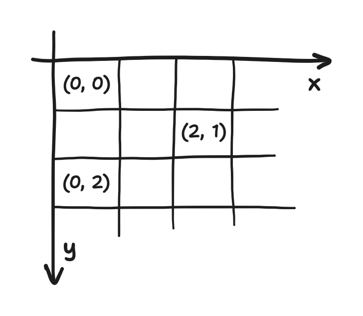
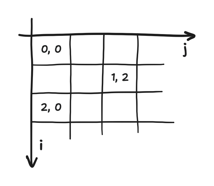
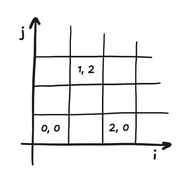
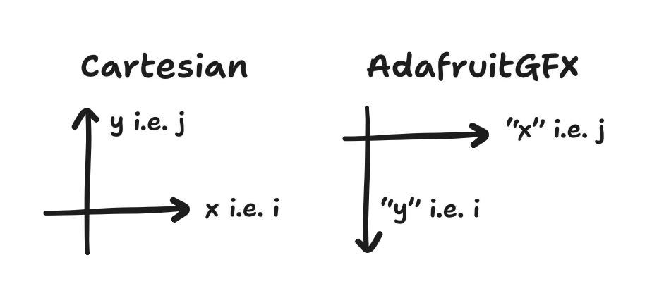
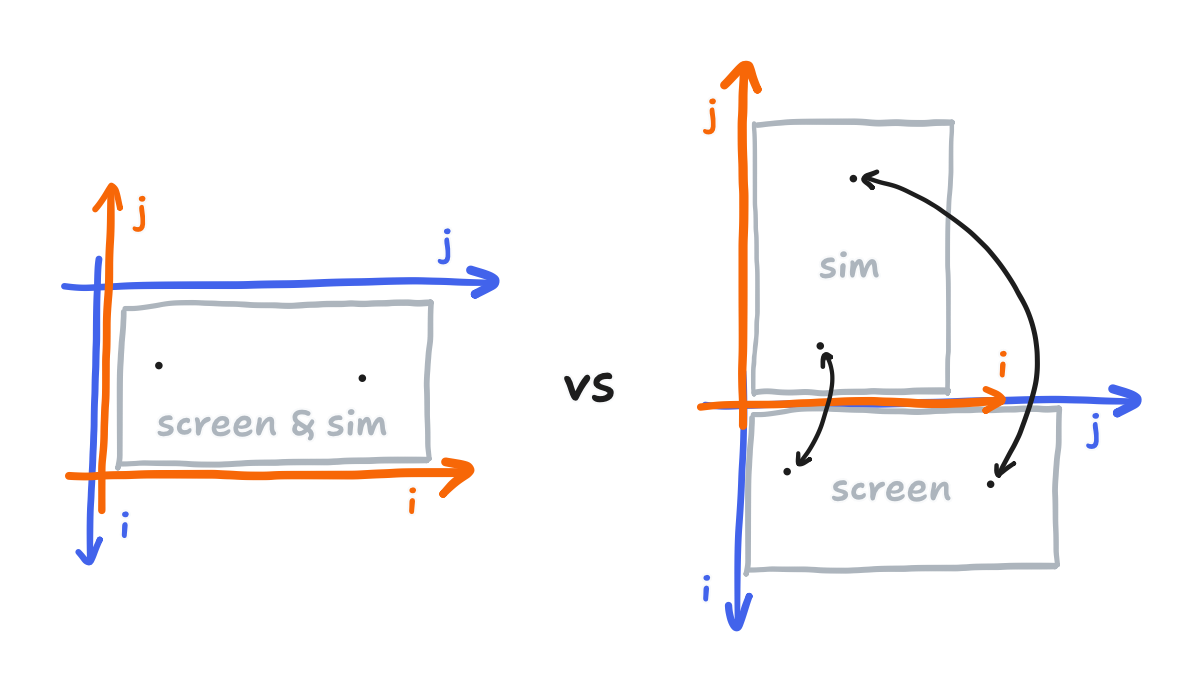
I mentioned in the last part that it is more useful to think of fields—which are arrays when discretized—as very long vectors. Where was I going with that, exactly? Our arrays are a 2D arrangement of data, with the position of each element neatly corresponding to a 2D location. Now, we care less for this correspondence when we’re doing the linear algebra. Vectors are a <em>1D</em> arrangement of data. To rearrange the array into a vector, convention tells us to read out the data like a book, increasing in <code class="language-plaintext highlighter-rouge">i</code> from left to right, then increasing in <code class="language-plaintext highlighter-rouge">j</code> from… bottom to top, actually, to stay within the Cartesian perspective. Once again, I already discussed the difference between matrix indexing and Cartesian indexing in Part 3. And of course, the conventional order isn’t the only order, and we’ll get to another one in this article soon enough.</p>

<p>Let’s make this concrete with an example. Consider a three-by-three grid and some scalar field $x$. Then, the discretization of $x$ on that grid is a three-by-three array. Reading out its elements gets a nine-element vector. All that is depicted below.</p>

<figure> 
<img src="/images/2024-09-26/figure9.png" alt="On the left, a three-by-three grid of squares, labelled from 1 to 9 in left-to-right then bottom-to-top order and overlayed with a zig-zag arrow going through the squares in said order. On the right, a vector containing the numbers 1 to 9 in increasing order. Between them, an arrow point from left to right." />
</figure>

<p>
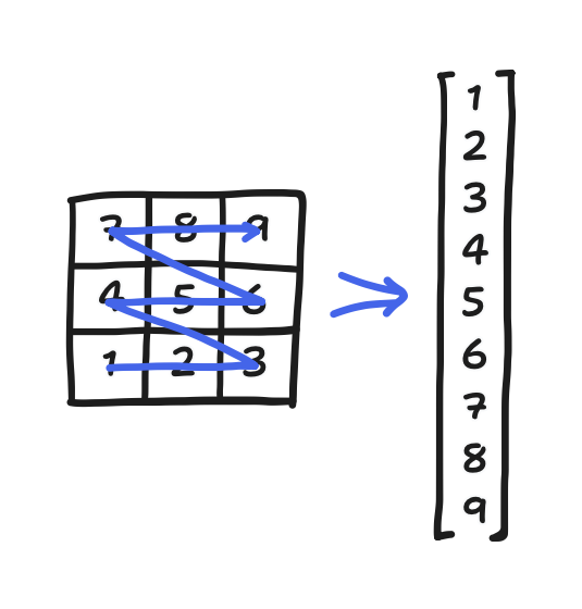
Let’s look at points 5 and 8. They’re right next to each other in 2D space, but now they’re so far apart on the vector! Such things happen with the conventional order.</p>

<p>More importantly, with arrays rearranged as vectors, we can show that our boundary value problem, when discretized the way we’ve done it, is a classic $Ax = b$ problem! If we let $x$ be the pressure vector and $b$ be the divergence, then the $i$-th row of $A$ represents the equation for <em>some specific point with location $i,\; j$</em> (yes, unfortunately $i$ and $j$ have double meanings here, one for indexing arrays/grids and one for indexing matrices), relating the $i$-th element of the divergence vector to the $i$-th element of the pressure vector, plus an element for each neighbor. Because of the conventional order, those neighbors would be the $(i+1)$-th, $(i-1)$-th, $(i+N)$-th, and $(i-N)$-th elements, where $N$ is the horizontal length of the array.</p>

<p>Let’s demonstrate this by determining the $A$ for our previous three-by-three example.</p>

<p>Starting from the governing equation, we can rewrite the left side so that the division by $\Delta x^2$ is multiplication by $\frac{1}{\Delta x^2}$.</p>

\[\frac{1}{\Delta x^2} \big( p[i + 1, j] + p[i - 1, j] + p[i, j + 1] + p[i, j - 1] - 4 p[i, j] \big) = d[i, j]\]

<p>This helps save some repetitive writing by defining $A = \frac{1}{\Delta x^2} B$, where $B$ just has the same coefficients as $A$ but with $\frac{1}{\Delta x^2}$ factored out.</p>

<p>Next, we recognize that, in a three-by-three matrix, $N = 3$. It follows that, for some given center $p[i, j]$ in the array, which maps to $p_i$ in the vector, getting the down neighbor $p[i, j - 1]$ is to get $p_{i - 3}$.</p>

<p>Let’s see this in action. The center element $i=1,\;j=1$ is the only element with all-real neighbors, so it stands for the typical case where the boundary conditions don’t apply. Following the conventional order, it’s the 5th element of the vector, $p_{5}$, and the governing equation here can be written as this.</p>

\[\frac{1}{\Delta x^2} \big( p_6 + p_4 + p_8 + p_2 - 4 p_5 \big) = d_5\]

<p>We can then fill in the corresponding row of $A$ like this:</p>

\[\frac{1}{\Delta x^2} \begin{bmatrix} \\ \\ \\ \\ 0 &amp; 1 &amp; 0 &amp; 1 &amp; -4 &amp; 1 &amp; 0 &amp; 1 &amp; 0 \\ \\ \\ \\ \! \end{bmatrix} \begin{bmatrix} p_1 \\ p_2 \\ p_3 \\ p_4 \\ p_5 \\ p_6 \\ p_7 \\ p_8 \\ p_9 \end{bmatrix} = \begin{bmatrix} d_1 \\ d_2 \\ d_3 \\ d_4 \\ d_5 \\ d_6 \\ d_7 \\ d_8 \\ d_9 \end{bmatrix}\]

<p>In this row, the element corresponding to $i=1,\;j=1$ itself gets a $-4$, the ones corresponding to its neighbors get a $1$, and all other elements get a zero. In general, because the discretized governing equation, being the instance of Poisson’s equation that it is, just relates the five elements of the pressure vector to an element of the divergence vector, <em>all</em> the coefficients for the other elements–the rest of the $i$-th row of $A$–must be zero. $A$ is sparse!</p>

<p>With that said, for the points along the boundary, some of those neighbors don’t exist, and as a result, their rows end up slightly different. For example, one step to the left lands us on $i = 0,\;j = 1$, which is on the left boundary, so applying our discretized Neumann boundary condition gets us this equation</p>

\[\frac{p[i+1, j] + p[i, j+1] + p[i, j-1] - 3 p[i, j]}{\Delta x^2} = d[i, j]\]

<p>where the terms canceling gets us this $-3$ instead of a $-4$. Following the same treatment as before, it’s corresponding row in $A$ looks like this:</p>

\[\frac{1}{\Delta x^2} \begin{bmatrix} \\ \\ \\ 1 &amp; 0 &amp; 0 &amp; -3 &amp; 1 &amp; 0 &amp; 1 &amp; 0 &amp; 0 \\ 0 &amp; 1 &amp; 0 &amp; 1 &amp; -4 &amp; 1 &amp; 0 &amp; 1 &amp; 0 \\ \\ \\ \\ \! \end{bmatrix} \begin{bmatrix} p_1 \\ p_2 \\ p_3 \\ p_4 \\ p_5 \\ p_6 \\ p_7 \\ p_8 \\ p_9 \end{bmatrix} = \begin{bmatrix} d_1 \\ d_2 \\ d_3 \\ d_4 \\ d_5 \\ d_6 \\ d_7 \\ d_8 \\ d_9 \end{bmatrix}\]

<p>One step up lands on $i = 0, \; j = 2$, which is on both the left and top boundary, and that gets us the following equation,</p>

\[\frac{p[i+1, j] + p[i, j-1] - 2 p[i, j]}{\Delta x^2} = d[i, j]\]

<p>and its corresponding row looks like this.</p>

\[\frac{1}{\Delta x^2} \begin{bmatrix} \\ \\ \\ 1 &amp; 0 &amp; 0 &amp; -3 &amp; 1 &amp; 0 &amp; 1 &amp; 0 &amp; 0 \\ 0 &amp; 1 &amp; 0 &amp; 1 &amp; -4 &amp; 1 &amp; 0 &amp; 1 &amp; 0 \\ \\ 0 &amp; 0 &amp; 0 &amp; 1 &amp; 0 &amp; 0 &amp; -2 &amp; 1 &amp; 0 \\ \\ \! \end{bmatrix} \begin{bmatrix} p_1 \\ p_2 \\ p_3 \\ p_4 \\ p_5 \\ p_6 \\ p_7 \\ p_8 \\ p_9 \end{bmatrix} = \begin{bmatrix} d_1 \\ d_2 \\ d_3 \\ d_4 \\ d_5 \\ d_6 \\ d_7 \\ d_8 \\ d_9 \end{bmatrix}\]

<p>All the possibilities—in the three-by-three example or in <em>any</em> size of screen—is covered by these cases after adjusting for whichever neighbors are in a ghost row/column. Let’s fill in the rest of $A$.</p>

\[\frac{1}{\Delta x^2} \begin{bmatrix} -2 &amp; 1 &amp; 0 &amp; 1 \\ 1 &amp; -3 &amp; 1 &amp; 0 &amp; 1 \\ 0 &amp; 1 &amp; -2 &amp; 0 &amp; 0 &amp; 1 \\ 1 &amp; 0 &amp; 0 &amp; -3 &amp; 1 &amp; 0 &amp; 1 \\ &amp; 1 &amp; 0 &amp; 1 &amp; -4 &amp; 1 &amp; 0 &amp; 1 \\ &amp; &amp; 1 &amp; 0 &amp; 1 &amp; -3 &amp; 0 &amp; 0 &amp; 1 \\ &amp; &amp; &amp; 1 &amp; 0 &amp; 0 &amp; -2 &amp; 1 &amp; 0 \\ &amp; &amp; &amp; &amp; 1 &amp; 0 &amp; 1 &amp; -3 &amp; 1 \\ &amp; &amp; &amp; &amp; &amp; 1 &amp; 0 &amp; 1 &amp; -2 \end{bmatrix} \begin{bmatrix} p_1 \\ p_2 \\ p_3 \\ p_4 \\ p_5 \\ p_6 \\ p_7 \\ p_8 \\ p_9 \end{bmatrix} = \begin{bmatrix} d_1 \\ d_2 \\ d_3 \\ d_4 \\ d_5 \\ d_6 \\ d_7 \\ d_8 \\ d_9 \end{bmatrix}\]

<p>Here, the empty elements are also zero. Blank elements are part of the typical notation for sparse matrices.</p>

<p>That completes this sketch of a specific $A$ and a description for how to construct $A$ for any particular grid. I should pause here for a moment and note that what we have so far is quite interesting. So far, we have</p>

<ul>
  <li>sought to achieve the incompressibility constraint using the Helmholtz-Hodge decomposition,</li>
  <li>found that we need to solve the supporting boundary value problem,</li>
  <li>applied a finite difference discretization to it, and</li>
  <li>arrived at just a case of $Ax = b$.</li>
</ul>

<p>When it comes to that $Ax = b$, $b$ takes from the divergence of the uncorrected velocity field, $x$ takes from the pressure field, and $A$ takes from the governing equation and the boundary conditions. Just by solving it for $x$, we find the pressure field that solves the boundary value problem. With that, the next step would be to use the Helmholtz-Hodge decomposition to extract out the divergence-free component of our velocity. Recall, that this means subtracting the gradient of the pressure from it. We implement this by subtracting the <em>discrete gradient</em>.</p>

\[v_x[i, j] = w_x[i, j] - \frac{p[i+1, j] - p[i-1, j]}{2 \Delta x}\]

\[v_y[i, j] = w_y[i, j] - \frac{p[i, j+1] - p[i, j-1]}{2 \Delta y}\]

<p>And with the divergence-free velocity, the incompressibility constraint is achieved, giving realistic, fluid-like motion. It’s a real problem in a problem in a problem! <em>But we still haven’t solved it yet</em>. Remember that the Helmholtz-Hodge decomposition tells us that the pressure field exists, but not how to find it. Let’s now talk about getting that done.</p>

<p>The expression of the boundary value problem as just a case of $Ax = b$ was part of the context I needed to know. In my first (failed) attempt to get a fluid sim on an ESP32, I only knew Stam’s “Real-Time Fluid Dynamics for Games”, Wong’s post, and the GPU Gems article. I got quite far on a PC, but it was no good on an ESP32. Those sources didn’t mention the $Ax = b$ explicitly. But now, you and I can discuss how to solve the problem using “Jacobi iteration” but also “Gauss-Seidel iteration” or “successive over-relaxation” (SOR). In general, these are “iterative methods”, computational routines that can be said to “converge” onto the solution. With enough number-crunching, one can get arbitrarily close to the solution, though they never get the solution exactly.</p>

<p>First, what is “Jacobi iteration”, and how does it apply?</p>

<p>$A$ is a square matrix. That comes from the pressure and divergence vectors being constructed from the same grid of points, thus having the same number of elements. Assuming $A$ is furthermore invertible (technically it’s not because we only have Neumann conditions, but we’ll get to that) then perhaps we could solve by calculating $A^{-1} b$. However, that’s an $O(N^3)$ operation—far too expensive, considering in this case that $N$ is the total number of points on the grid! To get something faster, we must exploit the sparsity of $A$, and Jacobi iteration happens to let us do that.</p>

<p>
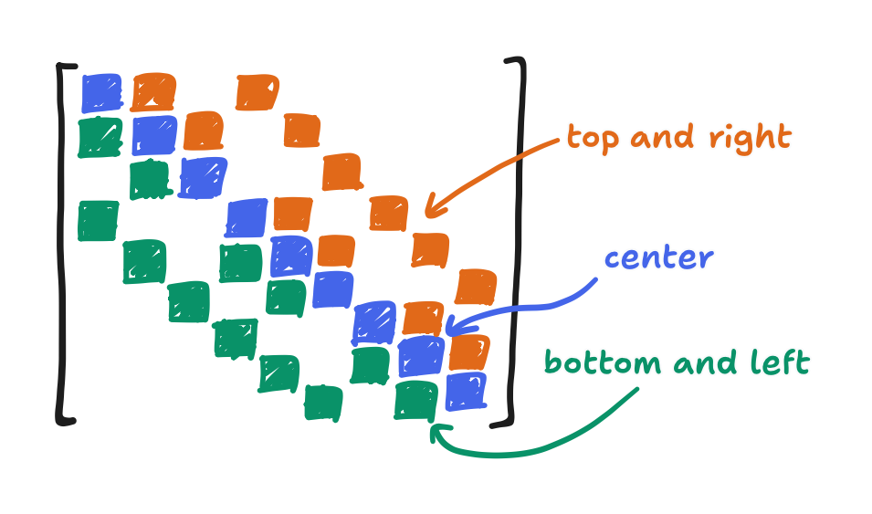
So, we start by expressing $A$ as the sum of (1) a cut-out of $A$ along the diagonal, hereby called $D$, and the rest of $A$, otherwise describable as (2) an upper-triangular part that we’ll call $U$ plus (3) a lower-triangular part we’ll call $L$.</p>

\[A = D + L + U\]

\[\begin{bmatrix} a_{11} &amp; a_{12} &amp; \cdots &amp; a_{1n} \\ a_{21} &amp; a_{22} &amp; \cdots &amp; a_{2n} \\ \vdots &amp; \vdots &amp; \ddots &amp; \vdots \\ a_{n1} &amp; a_{n2} &amp; \cdots &amp; a_{nn} \end{bmatrix} = \begin{bmatrix} a_{11} \\ &amp; a_{22} \\ &amp; &amp; \ddots \\ &amp; &amp; &amp; a_{nn} \end{bmatrix} + \begin{bmatrix} 0 \\ a_{21} &amp; 0 \\ a_{31} &amp; a_{32} &amp; 0 \\ \vdots &amp; \vdots &amp; \ddots &amp; \ddots \\ a_{n1} &amp; a_{n2} &amp; \cdots &amp; a_{n(n-1)} &amp; 0 \end{bmatrix} + \begin{bmatrix} 0 &amp; a_{12} &amp; a_{13} &amp; \cdots &amp; a_{1n} \\ &amp; 0 &amp; a_{23} &amp; \cdots &amp; a_{2n} \\ &amp; &amp; 0 &amp; \ddots &amp; \vdots \\ &amp; &amp; &amp; \ddots &amp; a_{(n-1)n} \\ &amp; &amp; &amp; &amp; 0 \end{bmatrix}\]

<p>Consider $a_{ij}$ where $i = j$, or in other words $a_{ii}$. The $i$-th point in the $i$-th row, which represents the governing equation centered at the $i$-th point, must always be the center. It follows that the diagonal cut-out $D$, which takes the elements $a_{ii}$, is taking the <em>coefficients of the centers</em>. That’s the $-4$’s, $-3$’s, and $-2$’s. Now consider how the conventional order is left-to-right then bottom-to-top. The lower-triangular cut-out $L$ contains all elements <em>preceding</em> the center. That is, it contains the left and bottom neighbors! The upper-triangular cut-out $U$ contains all elements <em>succeeding</em> the center i.e. the right and top neighbors!</p>

<figure> 
<img src="/images/2024-09-26/figure10.png" alt="An image made by filling in, with different colors, the lower-triangular (labeled as bottom and left), upper-triangular (labeled top and right), and diagonal (labeled center) parts of the given matrix A, from the three-by-three example." />
<figcaption>

What each entry in the $A$ of our three-by-three example means

</figcaption>
</figure>

<p>That aside, in this decomposition, it happens that $D$ is a diagonal matrix. As a result, we can say that its inverse $D^{-1}$ is just a matrix with <em>reciprocals</em> along the diagonal.</p>

\[D^{-1} = \begin{bmatrix} a_{11}^{-1} \\ &amp; a_{22}^{-1} \\ &amp; &amp; \ddots \\ &amp; &amp; &amp; a_{nn}^{-1} \end{bmatrix}\]

<p>With that in mind, we can derive the following equation from $Ax = b$,</p>

\[\begin{align*} A x &amp; = b \\ (D + L + U) x &amp; = b \\ Dx + (L+U)x &amp; = b \\ Dx &amp; = b - (L+U) x \\ x &amp; = D^{-1} (b - (L+U) x) \end{align*}\]

<p>where $x$ appears in two places. From there, Jacobi iteration is to let the right-hand $x$ be some guess at the solution that we’ll call $x^{(k)}$ and let the left-hand $x$ be the <em>updated</em> guess $x^{(k+1)}$.</p>

\[x^{(k+1)} = D^{-1} (b - (L+U) x^{(k)})\]

<p>In a moment, we’ll show that—given a specific condition holds—$x^{(k+1)}$ is <em>always</em> a better guess than $x^{(k)}$.</p>

<p>First, let’s see how the expression $D^{-1} (b - (L+U)x)$ manifests in practice. How is it faster than inverting $A$? Where do the sparse matrices come in? We just need to go get one element of $x^{(k+1)}$ at a time.</p>

<p>We know that $D^{-1}$, like $D$, is diagonal, and multiplying a vector by a diagonal matrix happens to be equivalent to multiplying each $i$-th element with its corresponding $a_{ii}^{-1}$.</p>

\[\begin{bmatrix} a_{11}^{-1} \\ &amp; a_{22}^{-1} \\ &amp; &amp; \ddots \\ &amp; &amp; &amp; a_{nn}^{-1} \end{bmatrix} \begin{bmatrix} x_1 \\ x_2 \\ \vdots \\ x_n \end{bmatrix} = \begin{bmatrix} a_{11}^{-1} x_1 \\ a_{22}^{-1} x_2 \\ \vdots \\ a_{nn}^{-1} x_n \end{bmatrix}\]

<p>So, to acquire some $i$-th element of $x^{(k+1)}$, we can at least compute $b - (L+U) x^{(k)}$ in its entirety, pick the $i$-th element of that, then multiply it by $a_{ii}^{-1}$. Next, to subtract $(L+U)x^{(k)}$ from $b$ is of course equivalent to subtracting each element of $(L+U)x^{(k)}$ from its corresponding element of $b$. That leaves $(L+U)x^{(k)}$ by itself.</p>

<p>Well, remember where we came from: $A$ is a sparse because each of its rows is just a discretized instance of Poisson’s equation. Said equation only involves the center point and its neighbors. If $D$ contained all the center coefficients, then $L+U$ is just the neighbor coefficients. That is, the $i$-th element of $(L+U)x^{(k)}$ is just a sum of the four neighbor terms.</p>

\[\frac{p[i+1, j] + p[i-1, j] + p[i, j+1] + p[i, j-1]}{\Delta x^2}\]

<div class="note-panel">

  <p>It’s a sum of the four neighbor terms when there <em>are</em> four of them, anyway. So that I may keep it concise, whenever you see a $-4$ and four terms, please adjust it to a $-3$ and three terms or $-2$ and two terms at the boundary.</p>

</div>

<p>From the bottom to the top, $D^{-1}(b-(L+U)x^{(k)})$ can be computed one element at a time. It’s a composition of three operations: multiplication by $a_{ii}^{-1}$, subtraction from $b_i$, and the summing of the neighbor terms. If we put it all together, we get this:</p>

\[p^{(k+1)}[i, j] = - \frac{\Delta x^2}{4} \left( d[i, j] - \frac{p^{(k)}[i+1, j] + p^{(k)}[i-1, j] + p^{(k)}[i, j+1] + p^{(k)}[i, j-1]}{\Delta x^2} \right)\]

<p>Apart from a bit of algebra, this is identical to the derivations of Jacobi iteration in Wong’s post and the GPU Gems article. Not bad!</p>

<p>Now, why is this fast? Generally speaking, if $A$ was not sparse, then a row of $(L+U)$ wouldn’t contain the four neighbors but rather $N$ terms, and as expected, the complexity of its dot product with $x$ is $O(N)$. Doing that for each of the $N$ rows of $A$ gives the expected complexity of a matrix-vector multiply, $O(N^2)$. Now, if a row had only four non-zero coefficients? And if we could just skip all the zeroes? The complexity of that dot product falls to $O(1)$, and the complexity of a matrix-vector multiply falls to $O(N)$–linear time! And given that it’s in the service of solving a $Ax = b$ problem, that’s <em>far</em> better than the expected $O(N^3)$! The catch: if we want to iterate as many times as it’ll take to achieve a fixed amount of improvement, <em>independent of the grid size</em>, the total complexity is higher. Really, true linear complexity lies in the domain of <a href="https://en.wikipedia.org/wiki/Multigrid_method">multigrid methods</a>, which is way outside when I’m familiar with and outside the scope of this article. We’ll instead iterate a fixed number of times and call it day.</p>

<p>Here’s what the code for that would look like. Please forgive my extensive use of pointers here.</p>

<div class="language-c highlighter-rouge"><div class="highlight"><pre class="highlight"><code><span class="k">struct</span> <span class="n">pois_context</span> <span class="p">{</span>
    <span class="kt">float</span> <span class="o">*</span><span class="n">d</span><span class="p">;</span>
    <span class="kt">float</span> <span class="n">dx</span><span class="p">;</span>
<span class="p">};</span>

<span class="k">static</span> <span class="kr">inline</span> <span class="kt">int</span> <span class="nf">index</span><span class="p">(</span><span class="kt">int</span> <span class="n">i</span><span class="p">,</span> <span class="kt">int</span> <span class="n">j</span><span class="p">,</span> <span class="kt">int</span> <span class="n">dim_x</span><span class="p">)</span> <span class="p">{</span>
    <span class="k">return</span> <span class="n">dim_x</span><span class="o">*</span><span class="n">j</span><span class="o">+</span><span class="n">i</span><span class="p">;</span>
<span class="p">}</span>

<span class="k">static</span> <span class="kt">float</span> <span class="nf">pois_expr_safe</span><span class="p">(</span><span class="kt">float</span> <span class="o">*</span><span class="n">p</span><span class="p">,</span> <span class="kt">int</span> <span class="n">i</span><span class="p">,</span> <span class="kt">int</span> <span class="n">j</span><span class="p">,</span> <span class="kt">int</span> <span class="n">dim_x</span><span class="p">,</span> <span class="kt">int</span> <span class="n">dim_y</span><span class="p">,</span>
        <span class="kt">void</span> <span class="o">*</span><span class="n">ctx</span><span class="p">)</span>
<span class="p">{</span>
    <span class="k">struct</span> <span class="n">pois_context</span> <span class="o">*</span><span class="n">pois_ctx</span> <span class="o">=</span> <span class="p">(</span><span class="k">struct</span> <span class="n">pois_context</span><span class="o">*</span><span class="p">)</span><span class="n">ctx</span><span class="p">;</span>
    <span class="kt">int</span> <span class="n">i_max</span> <span class="o">=</span> <span class="n">dim_x</span><span class="o">-</span><span class="mi">1</span><span class="p">,</span> <span class="n">j_max</span> <span class="o">=</span> <span class="n">dim_y</span><span class="o">-</span><span class="mi">1</span><span class="p">;</span>

    <span class="kt">float</span> <span class="n">p_sum</span> <span class="o">=</span> <span class="mi">0</span><span class="p">;</span>
    <span class="kt">int</span> <span class="n">a_ii</span> <span class="o">=</span> <span class="mi">0</span><span class="p">;</span>
    <span class="k">if</span> <span class="p">(</span><span class="n">i</span> <span class="o">&gt;</span> <span class="mi">0</span><span class="p">)</span> <span class="p">{</span>
        <span class="n">p_sum</span> <span class="o">+=</span> <span class="o">*</span><span class="p">(</span><span class="n">p</span><span class="o">-</span><span class="mi">1</span><span class="p">);</span>
        <span class="o">++</span><span class="n">a_ii</span><span class="p">;</span>
    <span class="p">}</span>
    <span class="k">if</span> <span class="p">(</span><span class="n">i</span> <span class="o">&lt;</span> <span class="n">i_max</span><span class="p">)</span> <span class="p">{</span>
        <span class="n">p_sum</span> <span class="o">+=</span> <span class="o">*</span><span class="p">(</span><span class="n">p</span><span class="o">+</span><span class="mi">1</span><span class="p">);</span>
        <span class="o">++</span><span class="n">a_ii</span><span class="p">;</span>
    <span class="p">}</span>
    <span class="k">if</span> <span class="p">(</span><span class="n">j</span> <span class="o">&gt;</span> <span class="mi">0</span><span class="p">)</span> <span class="p">{</span>
        <span class="n">p_sum</span> <span class="o">+=</span> <span class="o">*</span><span class="p">(</span><span class="n">p</span><span class="o">-</span><span class="n">dim_x</span><span class="p">);</span>
        <span class="o">++</span><span class="n">a_ii</span><span class="p">;</span>
    <span class="p">}</span>
    <span class="k">if</span> <span class="p">(</span><span class="n">j</span> <span class="o">&lt;</span> <span class="n">j_max</span><span class="p">)</span> <span class="p">{</span>
        <span class="n">p_sum</span> <span class="o">+=</span> <span class="o">*</span><span class="p">(</span><span class="n">p</span><span class="o">+</span><span class="n">dim_x</span><span class="p">);</span>
        <span class="o">++</span><span class="n">a_ii</span><span class="p">;</span>
    <span class="p">}</span>

    <span class="k">static</span> <span class="k">const</span> <span class="kt">float</span> <span class="n">neg_a_ii_inv</span><span class="p">[</span><span class="mi">5</span><span class="p">]</span> <span class="o">=</span> <span class="p">{</span><span class="mi">0</span><span class="p">,</span> <span class="mi">0</span><span class="p">,</span> <span class="o">-</span><span class="mi">1</span><span class="p">.</span><span class="mi">0</span><span class="o">/</span><span class="mi">2</span><span class="p">.</span><span class="mi">0</span><span class="p">,</span> <span class="o">-</span><span class="mi">1</span><span class="p">.</span><span class="mi">0</span><span class="o">/</span><span class="mi">3</span><span class="p">.</span><span class="mi">0</span><span class="p">,</span> <span class="o">-</span><span class="mi">1</span><span class="p">.</span><span class="mi">0</span><span class="o">/</span><span class="mi">4</span><span class="p">.</span><span class="mi">0</span><span class="p">};</span>
    <span class="kt">int</span> <span class="n">ij</span> <span class="o">=</span> <span class="n">index</span><span class="p">(</span><span class="n">i</span><span class="p">,</span> <span class="n">j</span><span class="p">,</span> <span class="n">dim_x</span><span class="p">);</span>

    <span class="k">return</span> <span class="n">neg_a_ii_inv</span><span class="p">[</span><span class="n">a_ii</span><span class="p">]</span> <span class="o">*</span> <span class="p">(</span><span class="n">pois_ctx</span><span class="o">-&gt;</span><span class="n">dx</span> <span class="o">*</span> <span class="n">pois_ctx</span><span class="o">-&gt;</span><span class="n">d</span><span class="p">[</span><span class="n">ij</span><span class="p">]</span> <span class="o">-</span> <span class="n">p_sum</span><span class="p">);</span>
<span class="p">}</span>

<span class="kt">void</span> <span class="nf">poisson_solve</span><span class="p">(</span><span class="kt">float</span> <span class="o">*</span><span class="n">p</span><span class="p">,</span> <span class="kt">float</span> <span class="o">*</span><span class="n">div</span><span class="p">,</span> <span class="kt">int</span> <span class="n">dim_x</span><span class="p">,</span> <span class="kt">int</span> <span class="n">dim_y</span><span class="p">,</span> <span class="kt">float</span> <span class="n">dx</span><span class="p">,</span>
        <span class="kt">int</span> <span class="n">iters</span><span class="p">,</span> <span class="kt">float</span> <span class="o">*</span><span class="n">scratch</span><span class="p">)</span>
<span class="p">{</span>
    <span class="kt">float</span> <span class="o">*</span><span class="n">wrt</span> <span class="o">=</span> <span class="n">p</span><span class="p">,</span> <span class="o">*</span><span class="n">rd</span> <span class="o">=</span> <span class="n">scratch</span><span class="p">,</span> <span class="o">*</span><span class="n">temp</span><span class="p">;</span>
    <span class="kt">int</span> <span class="n">ij</span><span class="p">;</span>

    <span class="k">for</span> <span class="p">(</span><span class="n">ij</span> <span class="o">=</span> <span class="mi">0</span><span class="p">;</span> <span class="n">ij</span> <span class="o">&lt;</span> <span class="n">dim_x</span><span class="o">*</span><span class="n">dim_y</span><span class="p">;</span> <span class="n">ij</span><span class="o">++</span><span class="p">)</span> <span class="p">{</span>
        <span class="n">p</span><span class="p">[</span><span class="n">ij</span><span class="p">]</span> <span class="o">=</span> <span class="mi">0</span><span class="p">;</span>
        <span class="n">scratch</span><span class="p">[</span><span class="n">ij</span><span class="p">]</span> <span class="o">=</span> <span class="mi">0</span><span class="p">;</span>
    <span class="p">}</span>

    <span class="k">struct</span> <span class="n">pois_context</span> <span class="n">pois_ctx</span> <span class="o">=</span> <span class="p">{.</span><span class="n">d</span> <span class="o">=</span> <span class="n">div</span><span class="p">,</span> <span class="p">.</span><span class="n">dims</span> <span class="o">=</span> <span class="n">dims</span><span class="p">,</span> <span class="p">.</span><span class="n">dx</span> <span class="o">=</span> <span class="n">dx</span><span class="p">};</span>

    <span class="k">for</span> <span class="p">(</span><span class="kt">int</span> <span class="n">k</span> <span class="o">=</span> <span class="mi">0</span><span class="p">;</span> <span class="n">k</span> <span class="o">&lt;</span> <span class="n">iters</span><span class="p">;</span> <span class="n">k</span><span class="o">++</span><span class="p">)</span> <span class="p">{</span>
        <span class="k">for</span> <span class="p">(</span><span class="kt">int</span> <span class="n">j</span> <span class="o">=</span> <span class="mi">0</span><span class="p">;</span> <span class="n">j</span> <span class="o">&lt;</span> <span class="n">dim_y</span><span class="p">;</span> <span class="n">j</span><span class="o">++</span><span class="p">)</span> <span class="p">{</span>
            <span class="k">for</span> <span class="p">(</span><span class="kt">int</span> <span class="n">i</span> <span class="o">=</span> <span class="mi">0</span><span class="p">;</span> <span class="n">i</span> <span class="o">&lt;</span> <span class="n">dim_x</span><span class="p">;</span> <span class="n">i</span><span class="o">++</span><span class="p">)</span> <span class="p">{</span>
                <span class="n">ij</span> <span class="o">=</span> <span class="n">index</span><span class="p">(</span><span class="n">i</span><span class="p">,</span> <span class="n">j</span><span class="p">,</span> <span class="n">dim_x</span><span class="p">);</span>
                <span class="n">wrt</span><span class="p">[</span><span class="n">ij</span><span class="p">]</span> <span class="o">=</span> <span class="n">pois_expr_safe</span><span class="p">(</span><span class="o">&amp;</span><span class="n">rd</span><span class="p">[</span><span class="n">ij</span><span class="p">],</span> <span class="n">i</span><span class="p">,</span> <span class="n">j</span><span class="p">,</span> <span class="n">dim_x</span><span class="p">,</span> <span class="n">dim_y</span><span class="p">,</span> <span class="o">&amp;</span><span class="n">pois_ctx</span><span class="p">);</span>
            <span class="p">}</span>
        <span class="p">}</span>
        <span class="n">temp</span> <span class="o">=</span> <span class="n">wrt</span><span class="p">;</span>
        <span class="n">wrt</span> <span class="o">=</span> <span class="n">rd</span><span class="p">;</span>
        <span class="n">rd</span> <span class="o">=</span> <span class="n">temp</span><span class="p">;</span>
    <span class="p">}</span>

    <span class="k">if</span> <span class="p">(</span><span class="n">wrt</span> <span class="o">==</span> <span class="n">scratch</span><span class="p">)</span> <span class="p">{</span>
        <span class="k">for</span> <span class="p">(</span><span class="n">ij</span> <span class="o">=</span> <span class="mi">0</span><span class="p">;</span> <span class="n">ij</span> <span class="o">&lt;</span> <span class="n">dim_x</span><span class="o">*</span><span class="n">dim_y</span><span class="p">;</span> <span class="n">ij</span><span class="o">++</span><span class="p">)</span> <span class="p">{</span>
            <span class="n">p</span><span class="p">[</span><span class="n">ij</span><span class="p">]</span> <span class="o">=</span> <span class="n">scratch</span><span class="p">[</span><span class="n">ij</span><span class="p">];</span>
        <span class="p">}</span>
    <span class="p">}</span>
<span class="p">}</span>
</code></pre></div></div>

<p>However! If we want to run this on an ESP32, that is too many if statements to be going through in the main loop. Instead, if we sweep through all the non-boundary elements first, we can skip those if statements. This creates a fast path.</p>

<p>Here’s what that looks like, on top of the previous code.</p>

<div class="language-c highlighter-rouge"><div class="highlight"><pre class="highlight"><code><span class="kt">void</span> <span class="nf">domain_iter</span><span class="p">(</span><span class="kt">float</span> <span class="p">(</span><span class="o">*</span><span class="n">expr_safe</span><span class="p">)(</span><span class="kt">float</span><span class="o">*</span><span class="p">,</span> <span class="kt">int</span><span class="p">,</span> <span class="kt">int</span><span class="p">,</span> <span class="kt">int</span><span class="p">,</span> <span class="kt">int</span><span class="p">,</span> <span class="kt">void</span><span class="o">*</span><span class="p">),</span>
        <span class="kt">float</span> <span class="p">(</span><span class="o">*</span><span class="n">expr_fast</span><span class="p">)(</span><span class="kt">float</span><span class="o">*</span><span class="p">,</span> <span class="kt">int</span><span class="p">,</span> <span class="kt">int</span><span class="p">,</span> <span class="kt">int</span><span class="p">,</span> <span class="kt">int</span><span class="p">,</span> <span class="kt">void</span><span class="o">*</span><span class="p">),</span> <span class="n">U</span> <span class="o">*</span><span class="n">wrt</span><span class="p">,</span>
        <span class="n">T</span> <span class="o">*</span><span class="n">rd</span><span class="p">,</span> <span class="kt">int</span> <span class="n">dim_x</span><span class="p">,</span> <span class="kt">int</span> <span class="n">dim_y</span><span class="p">,</span> <span class="kt">void</span> <span class="o">*</span><span class="n">ctx</span><span class="p">)</span>
<span class="p">{</span>
    <span class="kt">int</span> <span class="n">i_max</span> <span class="o">=</span> <span class="p">(</span><span class="n">dim_x</span><span class="p">)</span><span class="o">-</span><span class="mi">1</span><span class="p">,</span> <span class="n">j_max</span> <span class="o">=</span> <span class="p">(</span><span class="n">dim_y</span><span class="p">)</span><span class="o">-</span><span class="mi">1</span><span class="p">;</span>  <span class="c1">// inclusive!</span>
    <span class="kt">int</span> <span class="n">ij</span><span class="p">,</span> <span class="n">ij_alt</span><span class="p">;</span>

    <span class="c1">// Loop over the main body</span>
    <span class="k">for</span> <span class="p">(</span><span class="kt">int</span> <span class="n">j</span> <span class="o">=</span> <span class="mi">1</span><span class="p">;</span> <span class="n">j</span> <span class="o">&lt;</span> <span class="n">j_max</span><span class="p">;</span> <span class="o">++</span><span class="n">j</span><span class="p">)</span> <span class="p">{</span>
        <span class="k">for</span> <span class="p">(</span><span class="kt">int</span> <span class="n">i</span> <span class="o">=</span> <span class="mi">1</span><span class="p">;</span> <span class="n">i</span> <span class="o">&lt;</span> <span class="n">i_max</span><span class="p">;</span> <span class="o">++</span><span class="n">i</span><span class="p">)</span> <span class="p">{</span>
            <span class="n">ij</span> <span class="o">=</span> <span class="n">index</span><span class="p">(</span><span class="n">i</span><span class="p">,</span> <span class="n">j</span><span class="p">,</span> <span class="n">dim_x</span><span class="p">);</span>
            <span class="n">wrt</span><span class="p">[</span><span class="n">ij</span><span class="p">]</span> <span class="o">=</span> <span class="n">expr_fast</span><span class="p">(</span><span class="o">&amp;</span><span class="n">rd</span><span class="p">[</span><span class="n">ij</span><span class="p">],</span> <span class="n">i</span><span class="p">,</span> <span class="n">j</span><span class="p">,</span> <span class="n">dim_x</span><span class="p">,</span> <span class="n">dim_y</span><span class="p">,</span> <span class="n">ctx</span><span class="p">);</span>
        <span class="p">}</span>
    <span class="p">}</span>

    <span class="c1">// Loop over the top and bottom boundaries (including corners)</span>
    <span class="k">for</span> <span class="p">(</span><span class="kt">int</span> <span class="n">i</span> <span class="o">=</span> <span class="mi">0</span><span class="p">;</span> <span class="n">i</span> <span class="o">&lt;=</span> <span class="n">i_max</span><span class="p">;</span> <span class="o">++</span><span class="n">i</span><span class="p">)</span> <span class="p">{</span>
        <span class="n">ij</span> <span class="o">=</span> <span class="n">index</span><span class="p">(</span><span class="n">i</span><span class="p">,</span> <span class="mi">0</span><span class="p">,</span> <span class="n">dim_x</span><span class="p">);</span>
        <span class="n">wrt</span><span class="p">[</span><span class="n">ij</span><span class="p">]</span> <span class="o">=</span> <span class="n">expr_safe</span><span class="p">(</span><span class="o">&amp;</span><span class="n">rd</span><span class="p">[</span><span class="n">ij</span><span class="p">],</span> <span class="n">i</span><span class="p">,</span> <span class="mi">0</span><span class="p">,</span> <span class="n">dim_x</span><span class="p">,</span> <span class="n">dim_y</span><span class="p">,</span> <span class="n">ctx</span><span class="p">);</span>
        <span class="n">ij_alt</span> <span class="o">=</span> <span class="n">index</span><span class="p">(</span><span class="n">i</span><span class="p">,</span> <span class="n">j_max</span><span class="p">,</span> <span class="n">dim_x</span><span class="p">);</span>
        <span class="n">wrt</span><span class="p">[</span><span class="n">ij_alt</span><span class="p">]</span> <span class="o">=</span> <span class="n">expr_safe</span><span class="p">(</span><span class="o">&amp;</span><span class="n">rd</span><span class="p">[</span><span class="n">ij_alt</span><span class="p">],</span> <span class="n">i</span><span class="p">,</span> <span class="n">j_max</span><span class="p">,</span> <span class="n">dim_x</span><span class="p">,</span> <span class="n">dim_y</span><span class="p">,</span> <span class="n">ctx</span><span class="p">);</span>
    <span class="p">}</span>

    <span class="c1">// Loop over the left and right boundaries</span>
    <span class="k">for</span> <span class="p">(</span><span class="kt">int</span> <span class="n">j</span> <span class="o">=</span> <span class="mi">1</span><span class="p">;</span> <span class="n">j</span> <span class="o">&lt;</span> <span class="n">j_max</span><span class="p">;</span> <span class="o">++</span><span class="n">j</span><span class="p">)</span> <span class="p">{</span>
        <span class="n">ij</span> <span class="o">=</span> <span class="n">index</span><span class="p">(</span><span class="mi">0</span><span class="p">,</span> <span class="n">j</span><span class="p">,</span> <span class="n">dim_x</span><span class="p">);</span>
        <span class="n">wrt</span><span class="p">[</span><span class="n">ij</span><span class="p">]</span> <span class="o">=</span> <span class="n">expr_safe</span><span class="p">(</span><span class="o">&amp;</span><span class="n">rd</span><span class="p">[</span><span class="n">ij</span><span class="p">],</span> <span class="mi">0</span><span class="p">,</span> <span class="n">j</span><span class="p">,</span> <span class="n">dim_x</span><span class="p">,</span> <span class="n">dim_y</span><span class="p">,</span> <span class="n">ctx</span><span class="p">);</span>
        <span class="n">ij_alt</span> <span class="o">=</span> <span class="n">index</span><span class="p">(</span><span class="n">i_max</span><span class="p">,</span> <span class="n">j</span><span class="p">,</span> <span class="n">dim_x</span><span class="p">);</span>
        <span class="n">wrt</span><span class="p">[</span><span class="n">ij_alt</span><span class="p">]</span> <span class="o">=</span> <span class="n">expr_safe</span><span class="p">(</span><span class="o">&amp;</span><span class="n">rd</span><span class="p">[</span><span class="n">ij_alt</span><span class="p">],</span> <span class="n">i_max</span><span class="p">,</span> <span class="n">j</span><span class="p">,</span> <span class="n">dim_x</span><span class="p">,</span> <span class="n">dim_y</span><span class="p">,</span> <span class="n">ctx</span><span class="p">);</span>
    <span class="p">}</span>
<span class="p">}</span>

<span class="k">static</span> <span class="kt">float</span> <span class="nf">pois_expr_fast</span><span class="p">(</span><span class="kt">float</span> <span class="o">*</span><span class="n">p</span><span class="p">,</span> <span class="kt">int</span> <span class="n">i</span><span class="p">,</span> <span class="kt">int</span> <span class="n">j</span><span class="p">,</span> <span class="kt">int</span> <span class="n">dim_x</span><span class="p">,</span> <span class="kt">int</span> <span class="n">dim_y</span><span class="p">,</span>
        <span class="kt">void</span> <span class="o">*</span><span class="n">ctx</span><span class="p">)</span>
<span class="p">{</span>
    <span class="k">struct</span> <span class="n">pois_context</span> <span class="o">*</span><span class="n">pois_ctx</span> <span class="o">=</span> <span class="p">(</span><span class="k">struct</span> <span class="n">pois_context</span><span class="o">*</span><span class="p">)</span><span class="n">ctx</span><span class="p">;</span>

    <span class="kt">float</span> <span class="n">p_sum</span> <span class="o">=</span> <span class="p">((</span><span class="o">*</span><span class="p">(</span><span class="n">p</span><span class="o">-</span><span class="mi">1</span><span class="p">)</span> <span class="o">+</span> <span class="o">*</span><span class="p">(</span><span class="n">p</span><span class="o">+</span><span class="mi">1</span><span class="p">))</span> <span class="o">+</span> <span class="p">(</span><span class="o">*</span><span class="p">(</span><span class="n">p</span><span class="o">-</span><span class="n">dim_x</span><span class="p">)</span> <span class="o">+</span> <span class="o">*</span><span class="p">(</span><span class="n">p</span><span class="o">+</span><span class="n">dim_x</span><span class="p">)));</span>

    <span class="kt">int</span> <span class="n">ij</span> <span class="o">=</span> <span class="n">index</span><span class="p">(</span><span class="n">i</span><span class="p">,</span> <span class="n">j</span><span class="p">,</span> <span class="n">dim_x</span><span class="p">);</span>
    <span class="k">return</span> <span class="o">-</span><span class="mi">0</span><span class="p">.</span><span class="mi">25</span><span class="n">f</span> <span class="o">*</span> <span class="p">(</span><span class="n">pois_ctx</span><span class="o">-&gt;</span><span class="n">dx</span> <span class="o">*</span> <span class="n">pois_ctx</span><span class="o">-&gt;</span><span class="n">d</span><span class="p">[</span><span class="n">ij</span><span class="p">]</span> <span class="o">-</span> <span class="n">p_sum</span><span class="p">);</span>
<span class="p">}</span>

<span class="kt">void</span> <span class="nf">poisson_solve</span><span class="p">(</span><span class="kt">float</span> <span class="o">*</span><span class="n">p</span><span class="p">,</span> <span class="kt">float</span> <span class="o">*</span><span class="n">div</span><span class="p">,</span> <span class="kt">int</span> <span class="n">dim_x</span><span class="p">,</span> <span class="kt">int</span> <span class="n">dim_y</span><span class="p">,</span> <span class="kt">float</span> <span class="n">dx</span><span class="p">,</span>
        <span class="kt">int</span> <span class="n">iters</span><span class="p">,</span> <span class="kt">float</span> <span class="o">*</span><span class="n">scratch</span><span class="p">)</span>
<span class="p">{</span>
    <span class="kt">float</span> <span class="o">*</span><span class="n">wrt</span> <span class="o">=</span> <span class="n">p</span><span class="p">,</span> <span class="o">*</span><span class="n">rd</span> <span class="o">=</span> <span class="n">scratch</span><span class="p">,</span> <span class="o">*</span><span class="n">temp</span><span class="p">;</span>

    <span class="k">for</span> <span class="p">(</span><span class="kt">int</span> <span class="n">ij</span> <span class="o">=</span> <span class="mi">0</span><span class="p">;</span> <span class="n">ij</span> <span class="o">&lt;</span> <span class="n">dim_x</span><span class="o">*</span><span class="n">dim_y</span><span class="p">;</span> <span class="n">ij</span><span class="o">++</span><span class="p">)</span> <span class="p">{</span>
        <span class="n">p</span><span class="p">[</span><span class="n">ij</span><span class="p">]</span> <span class="o">=</span> <span class="mi">0</span><span class="p">;</span>
        <span class="n">scratch</span><span class="p">[</span><span class="n">ij</span><span class="p">]</span> <span class="o">=</span> <span class="mi">0</span><span class="p">;</span>
    <span class="p">}</span>

    <span class="k">struct</span> <span class="n">pois_context</span> <span class="n">pois_ctx</span> <span class="o">=</span> <span class="p">{.</span><span class="n">d</span> <span class="o">=</span> <span class="n">div</span><span class="p">,</span> <span class="p">.</span><span class="n">dims</span> <span class="o">=</span> <span class="n">dims</span><span class="p">,</span> <span class="p">.</span><span class="n">dx</span> <span class="o">=</span> <span class="n">dx</span><span class="p">};</span>

    <span class="k">for</span> <span class="p">(</span><span class="kt">int</span> <span class="n">k</span> <span class="o">=</span> <span class="mi">0</span><span class="p">;</span> <span class="n">k</span> <span class="o">&lt;</span> <span class="n">iters</span><span class="p">;</span> <span class="n">k</span><span class="o">++</span><span class="p">)</span> <span class="p">{</span>
        <span class="n">domain_iter</span><span class="p">(</span><span class="n">pois_expr_safe</span><span class="p">,</span> <span class="n">pois_expr_fast</span><span class="p">,</span> <span class="n">wrt</span><span class="p">,</span> <span class="n">rd</span><span class="p">,</span> <span class="n">dim_x</span><span class="p">,</span> <span class="n">dim_y</span><span class="p">,</span>
            <span class="o">&amp;</span><span class="n">pois_ctx</span><span class="p">);</span>
        <span class="n">temp</span> <span class="o">=</span> <span class="n">wrt</span><span class="p">;</span>
        <span class="n">wrt</span> <span class="o">=</span> <span class="n">rd</span><span class="p">;</span>
        <span class="n">rd</span> <span class="o">=</span> <span class="n">temp</span><span class="p">;</span>
    <span class="p">}</span>

    <span class="k">if</span> <span class="p">(</span><span class="n">wrt</span> <span class="o">==</span> <span class="n">scratch</span><span class="p">)</span> <span class="p">{</span>
        <span class="k">for</span> <span class="p">(</span><span class="kt">int</span> <span class="n">ij</span> <span class="o">=</span> <span class="mi">0</span><span class="p">;</span> <span class="n">ij</span> <span class="o">&lt;</span> <span class="n">dim_x</span><span class="o">*</span><span class="n">dim_y</span><span class="p">;</span> <span class="n">ij</span><span class="o">++</span><span class="p">)</span> <span class="p">{</span>
            <span class="n">p</span><span class="p">[</span><span class="n">ij</span><span class="p">]</span> <span class="o">=</span> <span class="n">scratch</span><span class="p">[</span><span class="n">ij</span><span class="p">];</span>
        <span class="p">}</span>
    <span class="p">}</span>
<span class="p">}</span>

</code></pre></div></div>

<p>That out of the way, why does the Jacobi method work in the first place?</p>

<p>Take the iteration rule and subtract the equation it comes from. Then, it reduces because the $b$ from each cancel.</p>

\[\begin{align*} &amp; &amp; x^{(k+1)} &amp; = D^{-1} (\cancel{b} - (L+U) x^{(k)} )\\ &amp; -( &amp; x &amp; = D^{-1} (\cancel{b} - (L+U) x) &amp; ) \\ \hline \\[-1em] &amp; &amp; x^{(k+1)} - x &amp; = - D^{-1} (L+U) (x^{(k)} - x) \end{align*}\]

<p>Consider what $x^{(k+1)}-x$ and $x^{(k)}-x$ mean. They’re the error of our guesses! With every iteration, this error is multiplied by $-D^{-1} (L+U)$! Let’s call this matrix $C_\text{Jac}$.</p>

<p>For ease of explanation, let’s assume that $C_\text{Jac}$ can be diagonalized (for the otherwise defective matrices, there’s another way to go about this that’s similar). Because it can be diagonalized, the error can be expressed as a linear combination of its eigenvectors,</p>

\[x^{(k)} - x = c_1^{(k)} v_1 + c_2^{(k)} v_2 + \dots + c_n^{(k)} v_n\]

<p>whereby each component gets multiplied by the corresponding eigenvalue in each iteration.</p>

\[\begin{align*} x^{(k+1)} - x &amp; = C_\text{Jac} (c_1^{(k)} v_1 + c_2^{(k)} v_2 + \dots + c_n^{(k)} v_n) \\ &amp; = c_1^{(k)} C_\text{Jac} v_1 + c_2^{(k)} C_\text{Jac} v_2 + \dots + c_n^{(k)} C_\text{Jac} v_n \\ &amp; = c_1^{(k)} \lambda_1 v_1 + c_2^{(k)} \lambda_2 v_2 + \dots + c_n^{(k)} \lambda_n v_n \end{align*}\]

<p>Let’s focus on a single term here—say $c_1^{(k)} \lambda_1 v_1$. On the next iteration, it gets multiplied by $C_\text{Jac}$ <em>again</em>, meaning that it becomes $c_1^{(k)} \lambda_1^2 v_1$. You can see that doing this repeatedly gets us an <em>exponential sequence</em>. The same can be said for the other terms. If any of the eigenvalues have a magnitude that is greater than one, then Jacobi iteration wouldn’t work because the error would explode. However, if all the eigenvalues have magnitudes that are less than one, then the error would converge to zero. The point: $x^{(k+1)}$ would always be a better guess than $x^{(k)}$.</p>

<p>The largest magnitude of all the eigenvalues is said to be the “spectral radius” of the matrix. Some of the eigenvalues having a magnitude over one is the same as the spectral radius being over one. <em>All</em> of them having a magnitude under one is the same as the spectral radius being under one. In the latter case, the eigenvector with the largest magnitude is decaying the slowest, but another way of looking at it is that all error decays at least as fast. For example, if the spectral radius of $C_\text{Jac}$ i.e. “$\rho(C_\text{Jac})$” is 0.9, then 20 iterations would multiply the error by 0.9 20 times. Actually working out what 0.9 to the 20th power is, we get about 0.12, or that the error is cut by about 88 percent. Going further to, say, 40 iterations, we get 0.014, or that the error is cut by 98.5 percent. We could keep going until the result is as accurate as needed. All-in-all, so long as the spectral radius is under one, Jacobi iteration can be used to solve our boundary value problem, giving the pressure field that appropriately fits the Helmholtz-Hodge decomposition.</p>

<p>That said, how can we know that it is? What is our spectral radius, actually? Well, about that…</p>

<p>I don’t know any proofs of one way or the other, but I just did provide a general—though not analytic—description of $A$. If we take some specific case of $A$, then there are iterative, sparse algorithms for (approximately) finding the eigenvalues and eigenvectors. In Python, the SciPy package offers one, <a href="https://docs.scipy.org/doc/scipy/reference/generated/scipy.sparse.linalg.eigs.html"><code class="language-plaintext highlighter-rouge">scipy.sparse.linalg.eigs</code></a>. Many months back, I thought that it would be perfect for finding the spectral radius. I wrote a script, and here it is.</p>

<div class="language-python highlighter-rouge"><div class="highlight"><pre class="highlight"><code><span class="kn">import</span> <span class="nn">numpy</span> <span class="k">as</span> <span class="n">np</span>
<span class="kn">from</span> <span class="nn">math</span> <span class="kn">import</span> <span class="n">prod</span>
<span class="kn">from</span> <span class="nn">matplotlib</span> <span class="kn">import</span> <span class="n">pyplot</span> <span class="k">as</span> <span class="n">plt</span>
<span class="kn">import</span> <span class="nn">scipy.linalg</span>
<span class="kn">from</span> <span class="nn">scipy.sparse</span> <span class="kn">import</span> <span class="n">csr_array</span><span class="p">,</span> <span class="n">eye</span>
<span class="kn">import</span> <span class="nn">scipy.sparse.linalg</span>

<span class="n">DX</span> <span class="o">=</span> <span class="mf">1.0</span>
<span class="n">N_EIGS</span> <span class="o">=</span> <span class="mi">20</span>
<span class="n">N_ROWS</span> <span class="o">=</span> <span class="mi">60</span>
<span class="n">N_COLS</span> <span class="o">=</span> <span class="mi">80</span>


<span class="k">def</span> <span class="nf">plot_eigs</span><span class="p">(</span>
    <span class="n">arr</span><span class="p">:</span> <span class="n">csr_array</span><span class="p">,</span> <span class="n">subplots</span><span class="p">:</span> <span class="nb">tuple</span><span class="p">[</span><span class="nb">int</span><span class="p">,</span> <span class="nb">int</span><span class="p">],</span> <span class="n">neg_first</span><span class="p">:</span> <span class="nb">bool</span> <span class="o">=</span> <span class="bp">True</span><span class="p">,</span> <span class="n">digits</span><span class="p">:</span> <span class="nb">int</span> <span class="o">=</span> <span class="mi">5</span>
<span class="p">):</span>
    <span class="n">n_eigs</span> <span class="o">=</span> <span class="n">prod</span><span class="p">(</span><span class="n">subplots</span><span class="p">)</span>

    <span class="n">eigs</span><span class="p">,</span> <span class="n">v</span> <span class="o">=</span> <span class="n">scipy</span><span class="p">.</span><span class="n">sparse</span><span class="p">.</span><span class="n">linalg</span><span class="p">.</span><span class="n">eigs</span><span class="p">(</span><span class="n">arr</span><span class="p">,</span> <span class="n">k</span><span class="o">=</span><span class="n">n_eigs</span><span class="p">,</span> <span class="n">which</span><span class="o">=</span><span class="s">"LM"</span><span class="p">)</span>

    <span class="c1"># I haven't seen non-real values, so don't show them for legibility
</span>    <span class="k">if</span> <span class="n">np</span><span class="p">.</span><span class="nb">any</span><span class="p">(</span><span class="n">np</span><span class="p">.</span><span class="n">imag</span><span class="p">(</span><span class="n">eigs</span><span class="p">))</span> <span class="ow">or</span> <span class="n">np</span><span class="p">.</span><span class="nb">any</span><span class="p">(</span><span class="n">np</span><span class="p">.</span><span class="n">imag</span><span class="p">(</span><span class="n">v</span><span class="p">)):</span>
        <span class="k">print</span><span class="p">(</span><span class="s">"warning: eigenvalues or eigenvectors have an imaginary component"</span><span class="p">)</span>
    <span class="n">eigs</span> <span class="o">=</span> <span class="n">np</span><span class="p">.</span><span class="n">real</span><span class="p">(</span><span class="n">eigs</span><span class="p">)</span>
    <span class="n">v</span> <span class="o">=</span> <span class="n">np</span><span class="p">.</span><span class="n">real</span><span class="p">(</span><span class="n">v</span><span class="p">)</span>

    <span class="c1"># round the eigenvalues for legibility, but check for ambiguity
</span>    <span class="n">eigs</span> <span class="o">=</span> <span class="n">np</span><span class="p">.</span><span class="nb">round</span><span class="p">(</span><span class="n">eigs</span><span class="p">,</span> <span class="n">digits</span><span class="p">)</span>
    <span class="n">pairwise_matches</span> <span class="o">=</span> <span class="n">np</span><span class="p">.</span><span class="n">count_nonzero</span><span class="p">(</span>
        <span class="n">eigs</span><span class="p">[:,</span> <span class="n">np</span><span class="p">.</span><span class="n">newaxis</span><span class="p">]</span> <span class="o">==</span> <span class="n">eigs</span><span class="p">[</span><span class="n">np</span><span class="p">.</span><span class="n">newaxis</span><span class="p">,</span> <span class="p">:],</span> <span class="n">axis</span><span class="o">=</span><span class="mi">1</span>
    <span class="p">)</span>
    <span class="k">if</span> <span class="n">np</span><span class="p">.</span><span class="nb">any</span><span class="p">((</span><span class="n">pairwise_matches</span> <span class="o">&gt;</span> <span class="mi">1</span><span class="p">)</span> <span class="o">&amp;</span> <span class="p">(</span><span class="n">eigs</span> <span class="o">!=</span> <span class="mi">0</span><span class="p">)):</span>  <span class="c1"># ignore self-match and zero
</span>        <span class="k">print</span><span class="p">(</span><span class="s">"warning: rounding has made some eigenvalues ambiguous"</span><span class="p">)</span>

    <span class="c1"># in case of a pos-neg pair, strictly show pos or neg first
</span>    <span class="n">is_pos</span> <span class="o">=</span> <span class="n">eigs</span> <span class="o">&gt;</span> <span class="mi">0</span>
    <span class="k">if</span> <span class="n">neg_first</span><span class="p">:</span>  <span class="c1"># pos first, then the stable descending sort flips that
</span>        <span class="n">eigs</span> <span class="o">=</span> <span class="n">np</span><span class="p">.</span><span class="n">hstack</span><span class="p">([</span><span class="n">eigs</span><span class="p">[</span><span class="n">is_pos</span><span class="p">],</span> <span class="n">eigs</span><span class="p">[</span><span class="o">~</span><span class="n">is_pos</span><span class="p">]])</span>
        <span class="n">v</span> <span class="o">=</span> <span class="n">np</span><span class="p">.</span><span class="n">hstack</span><span class="p">([</span><span class="n">v</span><span class="p">[:,</span> <span class="n">is_pos</span><span class="p">],</span> <span class="n">v</span><span class="p">[:,</span> <span class="o">~</span><span class="n">is_pos</span><span class="p">]])</span>
    <span class="k">else</span><span class="p">:</span>  <span class="c1"># neg first, then the stable descending sort flips that
</span>        <span class="n">eigs</span> <span class="o">=</span> <span class="n">np</span><span class="p">.</span><span class="n">hstack</span><span class="p">([</span><span class="n">eigs</span><span class="p">[</span><span class="o">~</span><span class="n">is_pos</span><span class="p">],</span> <span class="n">eigs</span><span class="p">[</span><span class="n">is_pos</span><span class="p">]])</span>
        <span class="n">v</span> <span class="o">=</span> <span class="n">np</span><span class="p">.</span><span class="n">hstack</span><span class="p">([</span><span class="n">v</span><span class="p">[:,</span> <span class="o">~</span><span class="n">is_pos</span><span class="p">],</span> <span class="n">v</span><span class="p">[:,</span> <span class="n">is_pos</span><span class="p">]])</span>
    <span class="n">permute</span> <span class="o">=</span> <span class="n">np</span><span class="p">.</span><span class="n">argsort</span><span class="p">(</span><span class="n">np</span><span class="p">.</span><span class="nb">abs</span><span class="p">(</span><span class="n">eigs</span><span class="p">),</span> <span class="n">stable</span><span class="o">=</span><span class="bp">True</span><span class="p">)[::</span><span class="o">-</span><span class="mi">1</span><span class="p">]</span>
    <span class="n">eigs</span> <span class="o">=</span> <span class="n">eigs</span><span class="p">[</span><span class="n">permute</span><span class="p">]</span>
    <span class="n">v</span> <span class="o">=</span> <span class="n">v</span><span class="p">[:,</span> <span class="n">permute</span><span class="p">]</span>

    <span class="n">MIN_RANGE</span> <span class="o">=</span> <span class="mf">1e-9</span>
    <span class="k">for</span> <span class="n">i</span> <span class="ow">in</span> <span class="nb">range</span><span class="p">(</span><span class="n">n_eigs</span><span class="p">):</span>
        <span class="n">eigenvector</span> <span class="o">=</span> <span class="n">v</span><span class="p">[:,</span> <span class="n">i</span><span class="p">].</span><span class="n">reshape</span><span class="p">((</span><span class="n">N_ROWS</span><span class="p">,</span> <span class="n">N_COLS</span><span class="p">))</span>
        <span class="n">v_min</span> <span class="o">=</span> <span class="n">np</span><span class="p">.</span><span class="nb">min</span><span class="p">(</span><span class="n">eigenvector</span><span class="p">)</span>
        <span class="n">v_max</span> <span class="o">=</span> <span class="n">np</span><span class="p">.</span><span class="nb">max</span><span class="p">(</span><span class="n">eigenvector</span><span class="p">)</span>
        <span class="k">if</span> <span class="n">v_max</span> <span class="o">-</span> <span class="n">v_min</span> <span class="o">&lt;</span> <span class="n">MIN_RANGE</span><span class="p">:</span>  <span class="c1"># probably a flat plane
</span>            <span class="n">v_max</span> <span class="o">+=</span> <span class="n">MIN_RANGE</span>
            <span class="n">v_min</span> <span class="o">-=</span> <span class="n">MIN_RANGE</span>
        <span class="n">plt</span><span class="p">.</span><span class="n">subplot</span><span class="p">(</span><span class="o">*</span><span class="n">subplots</span><span class="p">,</span> <span class="n">i</span><span class="o">+</span><span class="mi">1</span><span class="p">)</span>
        <span class="n">plt</span><span class="p">.</span><span class="n">imshow</span><span class="p">(</span><span class="n">eigenvector</span><span class="p">,</span> <span class="n">vmin</span><span class="o">=</span><span class="n">v_min</span><span class="p">,</span> <span class="n">vmax</span><span class="o">=</span><span class="n">v_max</span><span class="p">,</span> <span class="n">cmap</span><span class="o">=</span><span class="s">"coolwarm"</span><span class="p">)</span>
        <span class="n">plt</span><span class="p">.</span><span class="n">axis</span><span class="p">(</span><span class="s">"off"</span><span class="p">)</span>
        <span class="n">plt</span><span class="p">.</span><span class="n">title</span><span class="p">(</span><span class="s">'$</span><span class="se">\\</span><span class="s">lambda$ = %0.*f'</span> <span class="o">%</span> <span class="p">(</span><span class="n">digits</span><span class="p">,</span> <span class="n">eigs</span><span class="p">[</span><span class="n">i</span><span class="p">]))</span>

    <span class="n">plt</span><span class="p">.</span><span class="n">tight_layout</span><span class="p">()</span>


<span class="n">op</span> <span class="o">=</span> <span class="n">scipy</span><span class="p">.</span><span class="n">sparse</span><span class="p">.</span><span class="n">linalg</span><span class="p">.</span><span class="n">LaplacianNd</span><span class="p">((</span><span class="n">N_ROWS</span><span class="p">,</span> <span class="n">N_COLS</span><span class="p">),</span> <span class="n">boundary_conditions</span><span class="o">=</span><span class="s">"neumann"</span><span class="p">)</span>
<span class="n">arr</span> <span class="o">=</span> <span class="p">(</span><span class="mi">1</span> <span class="o">/</span> <span class="p">(</span><span class="n">DX</span> <span class="o">**</span> <span class="mi">2</span><span class="p">))</span> <span class="o">*</span> <span class="n">csr_array</span><span class="p">(</span><span class="n">op</span><span class="p">.</span><span class="n">tosparse</span><span class="p">(),</span> <span class="n">dtype</span><span class="o">=</span><span class="n">np</span><span class="p">.</span><span class="n">float64</span><span class="p">)</span>

<span class="c1"># Jacobi
</span><span class="n">diag_inv</span> <span class="o">=</span> <span class="n">arr</span><span class="p">.</span><span class="n">diagonal</span><span class="p">(</span><span class="mi">0</span><span class="p">)</span> <span class="o">**</span> <span class="o">-</span><span class="mi">1</span>
<span class="n">lu</span> <span class="o">=</span> <span class="n">arr</span><span class="p">.</span><span class="n">copy</span><span class="p">()</span>
<span class="n">lu</span><span class="p">.</span><span class="n">setdiag</span><span class="p">(</span><span class="mi">0</span><span class="p">,</span> <span class="mi">0</span><span class="p">)</span>
<span class="n">iter_matrix_jacobi</span> <span class="o">=</span> <span class="n">diag_inv</span><span class="p">[:,</span> <span class="n">np</span><span class="p">.</span><span class="n">newaxis</span><span class="p">]</span> <span class="o">*</span> <span class="n">lu</span>  <span class="c1"># implements D^(-1) (L + U)
</span><span class="n">plot_eigs</span><span class="p">(</span><span class="n">iter_matrix_jacobi</span><span class="p">,</span> <span class="p">(</span><span class="mi">3</span><span class="p">,</span> <span class="mi">4</span><span class="p">),</span> <span class="n">neg_first</span><span class="o">=</span><span class="bp">True</span><span class="p">)</span>
<span class="n">plt</span><span class="p">.</span><span class="n">savefig</span><span class="p">(</span><span class="s">"eigs_jacobi.png"</span><span class="p">,</span> <span class="n">dpi</span><span class="o">=</span><span class="mi">300</span><span class="p">)</span>
<span class="n">plt</span><span class="p">.</span><span class="n">cla</span><span class="p">()</span>

<span class="c1"># Richardson
</span><span class="n">omega</span> <span class="o">=</span> <span class="p">(</span><span class="n">DX</span> <span class="o">**</span> <span class="mi">2</span><span class="p">)</span> <span class="o">/</span> <span class="o">-</span><span class="mi">4</span>
<span class="n">iter_matrix_richardson</span> <span class="o">=</span> <span class="n">csr_array</span><span class="p">(</span><span class="n">eye</span><span class="p">(</span><span class="n">arr</span><span class="p">.</span><span class="n">shape</span><span class="p">[</span><span class="mi">0</span><span class="p">]),</span> <span class="n">dtype</span><span class="o">=</span><span class="n">np</span><span class="p">.</span><span class="n">float64</span><span class="p">)</span> <span class="o">-</span> <span class="n">omega</span> <span class="o">*</span> <span class="n">arr</span>
<span class="n">plot_eigs</span><span class="p">(</span><span class="n">iter_matrix_richardson</span><span class="p">,</span> <span class="p">(</span><span class="mi">3</span><span class="p">,</span> <span class="mi">4</span><span class="p">),</span> <span class="bp">False</span><span class="p">)</span>
<span class="n">plt</span><span class="p">.</span><span class="n">savefig</span><span class="p">(</span><span class="s">"eigs_richardson.png"</span><span class="p">,</span> <span class="n">dpi</span><span class="o">=</span><span class="mi">300</span><span class="p">)</span>
<span class="n">plt</span><span class="p">.</span><span class="n">cla</span><span class="p">()</span>
</code></pre></div></div>

<p>
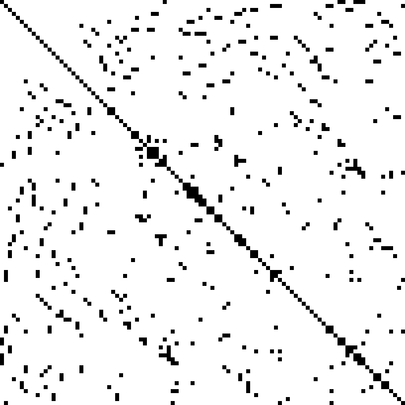
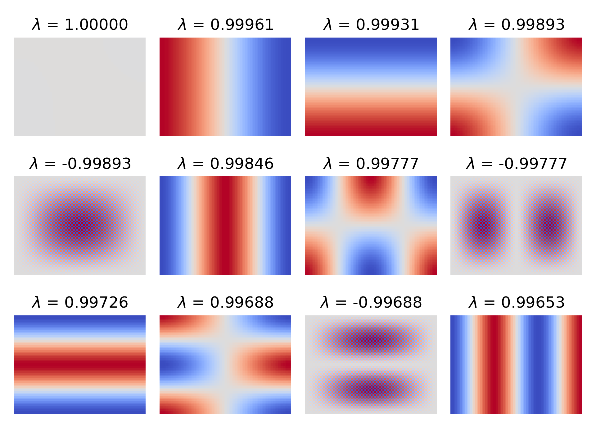
Given some $\Delta x$ and some grid, it calculates $A$, calculates $C_\text{Jac}$ from $A$ (and $C_\text{Richardson}$, but we’ll get to that) then finds the top twenty eigenvalues with the largest magnitude—plus the corresponding eigenvectors. Then, the spectral radius is just taking the first largest magnitude. It’s not useful for making a general statement about all cases of $A$, but it’s all I need for my specific case. I also went ahead here and reshaped the eigenvectors back into arrays, letting us visualize whatever eigenvector getting hit with so-and-so eigenvalue as <em>the component of a field</em> getting diminished.</p>

<p>In the case of ESP32-fluid-simulation, I was limited by the ESP32’s RAM to a $60 \times 80$ grid, and I happened to let $\Delta x = 1$. Given that, the script got this:</p>

<figure> 
<img src="/images/2024-09-26/figure11.png" alt="A range of image plots, each showing the component of the error associated with an eigenvalue, sorted in order of decreasing magnitude. The image plots for poitive eigenvalues appear to be checkered versions of the plots for the negative values." />
<figcaption>

Note: red is positive and blue is negative.

</figcaption>
</figure>

<p>
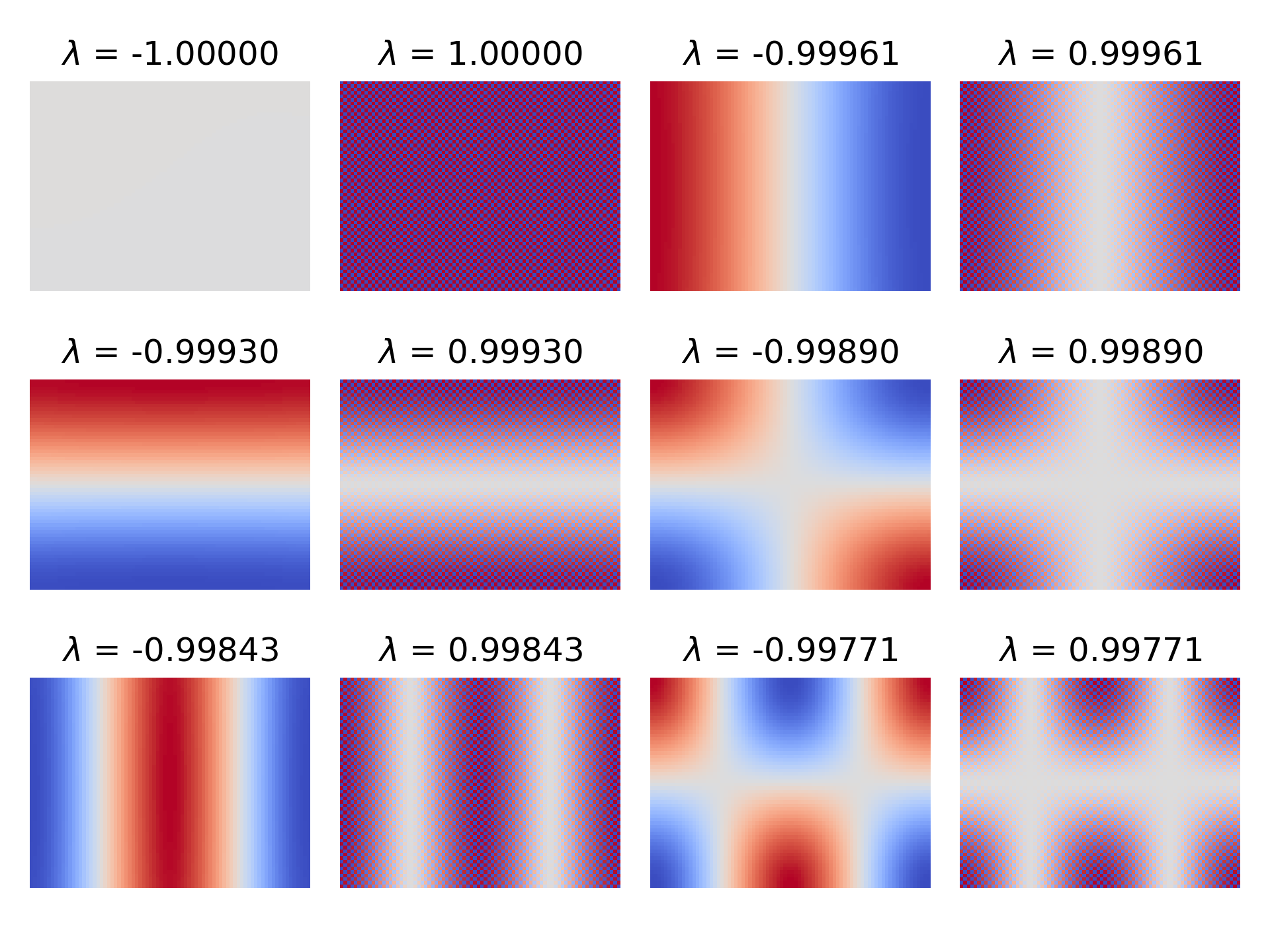
Immediately, we can notice two things:</p>

<ol>
  <li>
    <p>The spectral radius of $C_\text{Jac}$ appears to be <em>not</em> less than one because two of the eigenvalues are $1$ and $-1$.</p>
  </li>
  <li>
    <p>There seems to be positive-negative pairs of eigenvalues, with the eigenvector associated with the positive one looking like the negative counterpart but multiplied by a checkerboard pattern.</p>
  </li>
</ol>

<p>From what I’ve gathered, both of these things are to be expected.</p>

<p>Regarding (2), following linked references on Wikipedia led me to a 1950 PhD thesis by David M. Young—an analysis of “successive over-relaxation” in the context of finite difference schemes. Setting aside what “successive over-relaxation” is for now, I worked out that $A$ happens to satisfy what Young calls “property A”. In fact, Young was deriving results from this “property A” with a finite difference problem like this in mind! The thesis is <a href="https://www.stat.uchicago.edu/~lekheng/courses/324/young.pdf">publicly available</a> if you want to see how Young describes it exactly, but in this context, it’s this: given $A$ only has points interact with their neighbors, the grid can be divided into a succession of sets of points where each set only interacts with the preceding and the succeeding set.</p>

<figure> 
<img src="/images/2024-09-26/figure12.png" alt="A three-by-five grid of squares, numbered as follows: the top left square is labeled with one, the bottom and right neigbors of that square are labeled with two, all the bottom and right neighbors are in turn labeled with three, then proceeding onward like a wave until the bottom-right corner is reached." />
<figcaption>

The numbering of a three-by-five grid that works toward satisfying property A. Notice how a point labeled "three" only has points labeled "two" and "four" for neighbors.

</figcaption>
</figure>

<p>Because property A is satisfied, much of the conclusions of that analysis follow. That includes a theorem that states that the eigenvalues of Jacobi iteration (which he called the “Kormes method”, apparently) will come in positive-negative pairs, associated with a pair of eigenvectors where one is just a copy of the other but multiplied by $1$ and $-1$ alternating. That’s exactly what we’re seeing here!</p>

<p>As you might expect, we’ll be interested in Property A and “successive over-relaxation” soon.</p>

<p>Regarding (1), I found a <a href="https://scicomp.stackexchange.com/questions/21612/poisson-equation-finite-difference-with-pure-neumann-boundary-conditions">Stack Exchange</a> post that states that an $A$ constructed from a boundary value problem with only i.e. “purely” Neumann boundaries must have infinitely many solutions, separated by a constant, because the entire boundary value problem, which is just the governing equations (which are partial differential equations) and the boundary conditions, then only concerns the <em>derivative</em> of the pressure field. It’s like tacking on “$+\;C$” to the end of an indefinite integral’s result. That means there needs to be a place to <em>choose</em> that constant.</p>

<p>Looking at the eigenvector corresponding to $-1$: it’s very flat. As a flat component that doesn’t diminish over iterations, it looks to me like setting the initial weight of this component is equivalent to choosing the constant part of the solution.</p>

<p>In my case, I always started with a zeroed-out field as the first guess, which zeroes out that component too. But in any case, the neat part is that the choice of constant <em>doesn’t matter</em> because we ultimately subtract the <em>gradient</em> of the pressure from the uncorrected velocity. The gradient consists of partial derivatives, and the constant part doesn’t change its value. The same can be said for its checkerboard counterpart because the discrete gradient, using central differences, always happens to use points with the same color, so to speak. In other words, we’re free to take the <em>next largest</em> eigenvalue as our “spectral radius”—to abuse the term a bit. For our 60 x 80 grid (and a $\Delta x$ of 1), that’s 0.9996. Since “spectral radius” is less than one, we can be sure that Jacobi iteration solves this particular boundary value problem.</p>

<div class="note-panel">

  <p>One more “but actually” before we move on: I mentioned that my script can also calculate $C_\text{Richardson}$. I noticed in my sources that their codes for computing “Jacobi” iteration element-wise didn’t exactly do $D^{-1} (b - (L+U) x^{(k)})$. When it came time to multiply by $a_{ii}^{-1}$, which can be either $-\frac{\Delta x^2}{4}$, $-\frac{\Delta x^2}{3}$, or $-\frac{\Delta x^2}{2}$ depending on whether the $i$-th point is at the boundary, they just always multiplied by $-\frac{\Delta x^2}{4}$ instead. At the same time, instead of making sure to not take the top neighbor at the top boundary, left neighbor at the left boundary, et cetera, they pulled the ghost row/column value instead. I realized later that this was technically Richardson iteration.</p>

  <p>Richardson iteration comes from a different splitting of $A$ into a diagonal matrix of <em>constants</em> and the remainder.</p>

\[A = \alpha I + (A - \alpha I)\]

  <p>With this sum, we can do the following derivation from $Ax = b$, like we did for Jacobi iteration.</p>

\[\begin{align*} Ax &amp; = b \\ (\alpha I + (A - \alpha I)) x &amp; = b \\ \alpha I x + (A - \alpha I) x &amp; = b \\ \alpha I x &amp; = b - (A - \alpha I) x \\ x &amp; = \alpha^{-1} I (b - (A - \alpha I)x) \\ &amp; = \alpha^{-1} b - \alpha^{-1} (A - \alpha I) x \\ &amp; = \alpha^{-1} b + (I - \alpha^{-1} A) x \\ &amp; \left\downarrow \text{Let }\omega = \alpha^{-1} \right. \\ &amp; = \omega b + (I - \omega A) x\end{align*}\]

  <p>We can also turn that into the following iteration rule.</p>

\[x^{(k+1)} = \omega b + (I - \omega A) x^{(k)}\]

  <p>Consider letting $\alpha = \frac{-4}{\Delta x^2}$ (conversely $\omega = \frac{\Delta x^2}{-4}$) so that $\alpha$ is exactly $a_{ii}$ if all four neighbors were there. Then, if $\alpha I$ is subtracted from $A$, a zero remains where $a_{ii}$ once was. Now, notice in the derivation how $(A - \alpha I)$ times $-\alpha^{-1}$ is $I - \omega A$. If there was a zero on the diagonal of $(A - \alpha I)$, there’s still a zero there in $I - \omega A$. This says the pressure at the center isn’t in play, like how it’s not in Jacobi iteration. Overall, it can be shown that Richardson iteration and Jacobi iteration happen to be identical in our problem, <em>except</em> at the boundary.</p>

  <p>There, $a_{ii}$ is $\frac{-3}{\Delta x^2}$ or $\frac{-2}{\Delta x^2}$, and $-\frac{1}{4}$ or $-\frac{2}{4}$ is left, not zero, and so the pressure at the center point gets pulled in. When this is compared to how Stam’s “Real-Time Fluid Dynamics for Games” and the GPU Gems article pull a value from the ghost row/column, which in turn pulls from the center, it can be shown that what they’re doing is actually Richardson iteration! (Stam doesn’t do Richardson iteration to the tee, but we’ll get to that.)</p>

  <p>When it comes to code, those articles proceed to use the ghost rows and columns as actual rows and columns in memory that are kept up-to-date. That lets them use the fast path on <em>every</em> point because every point does then have all four “neighbors”. This also has the same function run on all points, which is important for GPUs. But for us, that idea is incompatible with the C code I’ve shown so far. At the very least, Richardson iteration could still be achieved by updating the safe path code, and we wouldn’t need to update the fast path code because that part is the same.</p>

  <div class="language-c highlighter-rouge"><div class="highlight"><pre class="highlight"><code><span class="k">static</span> <span class="kt">float</span> <span class="nf">pois_expr_safe</span><span class="p">(</span><span class="kt">float</span> <span class="o">*</span><span class="n">p</span><span class="p">,</span> <span class="kt">int</span> <span class="n">i</span><span class="p">,</span> <span class="kt">int</span> <span class="n">j</span><span class="p">,</span> <span class="kt">int</span> <span class="n">dim_x</span><span class="p">,</span> <span class="kt">int</span> <span class="n">dim_y</span><span class="p">,</span>
        <span class="kt">void</span> <span class="o">*</span><span class="n">ctx</span><span class="p">)</span>
<span class="p">{</span>
    <span class="k">struct</span> <span class="n">pois_context</span> <span class="o">*</span><span class="n">pois_ctx</span> <span class="o">=</span> <span class="p">(</span><span class="k">struct</span> <span class="n">pois_context</span><span class="o">*</span><span class="p">)</span><span class="n">ctx</span><span class="p">;</span>
    <span class="kt">int</span> <span class="n">i_max</span> <span class="o">=</span> <span class="n">dim_x</span><span class="o">-</span><span class="mi">1</span><span class="p">,</span> <span class="n">j_max</span> <span class="o">=</span> <span class="n">dim_y</span><span class="o">-</span><span class="mi">1</span><span class="p">;</span>

    <span class="kt">float</span> <span class="n">p_sum</span> <span class="o">=</span> <span class="mi">0</span><span class="p">;</span>
    <span class="n">p_sum</span> <span class="o">+=</span> <span class="p">(</span><span class="n">i</span> <span class="o">&gt;</span> <span class="mi">0</span><span class="p">)</span> <span class="o">?</span> <span class="o">*</span><span class="p">(</span><span class="n">p</span><span class="o">-</span><span class="mi">1</span><span class="p">)</span> <span class="o">:</span> <span class="o">*</span><span class="n">p</span><span class="p">;</span>
    <span class="n">p_sum</span> <span class="o">+=</span> <span class="p">(</span><span class="n">i</span> <span class="o">&lt;</span> <span class="n">i_max</span><span class="p">)</span> <span class="o">?</span> <span class="o">*</span><span class="p">(</span><span class="n">p</span><span class="o">+</span><span class="mi">1</span><span class="p">)</span> <span class="o">:</span> <span class="o">*</span><span class="n">p</span><span class="p">;</span>
    <span class="n">p_sum</span> <span class="o">+=</span> <span class="p">(</span><span class="n">j</span> <span class="o">&gt;</span> <span class="mi">0</span><span class="p">)</span> <span class="o">?</span> <span class="o">*</span><span class="p">(</span><span class="n">p</span><span class="o">-</span><span class="n">dim_x</span><span class="p">)</span> <span class="o">:</span> <span class="o">*</span><span class="n">p</span><span class="p">;</span>
    <span class="n">p_sum</span> <span class="o">+=</span> <span class="p">(</span><span class="n">j</span> <span class="o">&lt;</span> <span class="n">j_max</span><span class="p">)</span> <span class="o">?</span> <span class="o">*</span><span class="p">(</span><span class="n">p</span><span class="o">+</span><span class="n">dim_x</span><span class="p">)</span> <span class="o">:</span> <span class="o">*</span><span class="n">p</span><span class="p">;</span>

    <span class="kt">int</span> <span class="n">ij</span> <span class="o">=</span> <span class="n">INDEX</span><span class="p">(</span><span class="n">i</span><span class="p">,</span> <span class="n">j</span><span class="p">,</span> <span class="n">dim_x</span><span class="p">);</span>
    <span class="k">return</span> <span class="o">-</span><span class="mi">0</span><span class="p">.</span><span class="mi">25</span> <span class="o">*</span> <span class="p">(</span><span class="n">pois_ctx</span><span class="o">-&gt;</span><span class="n">dx</span> <span class="o">*</span> <span class="n">pois_ctx</span><span class="o">-&gt;</span><span class="n">d</span><span class="p">[</span><span class="n">ij</span><span class="p">]</span> <span class="o">-</span> <span class="n">p_sum</span><span class="p">);</span>
<span class="p">}</span>
</code></pre></div>  </div>

  <p>To be clear, this function wouldn’t work in my current code. It relies on the ghost rows and columns becoming actual, allocated memory, being constantly updated with the values of the real rows and columns in between iterations.</p>

  <p>That’s beside the point that I wanted to make, though. Since they actually used Richardson iteration, I wanted to make sure that the spectral radius of $C_\text{Richardson}$ was also under one, so I added on to the script. To do that, I just needed to know what matrix the error gets multiplied by, and we can use the same equation subtraction as before to find that it’s $(I - \omega A)$.</p>

\[\begin{align*} &amp; &amp; x^{(k+1)} &amp; = \cancel{\omega b} + (I - \omega A) x^{(k)}\\ &amp; -( &amp; x &amp; = \cancel{\omega b} + (I - \omega A) x &amp; ) \\ \hline \\[-1em] &amp; &amp; x^{(k+1)} - x &amp; = (I - \omega A) (x^{(k)} - x) \end{align*}\]

  <p>Here’s its eigenvalues and eigenvectors for the $60 \times 80$ grid and $\Delta x = 1$:</p>

  <figure> 
<img src="/images/2024-09-26/figure13.png" alt="A range of image plots, each showing the component of the error associated with an eigenvalue, sorted in order of decreasing magnitude. The image plots for poitive eigenvalues appear to be checkered versions of the plots for the negative values." />
</figure>

  <p>Though the eigenvectors are somewhat different, the spectral radius is completely within rounding error to that of Jacobi iteration in this case. It makes sense, given that $-\frac{4}{\Delta x^2}$ was the typical value on the diagonal. So, I wouldn’t be so concerned with the distinction, but I know I should at least point it out.</p>

</div>

<p>By showing exactly how Jacobi iteration manifests into code via sparse matrices and discussing the spectral radius, we’ve covered all the context that I once used to go <em>beyond</em>. Let’s start with a motivating question: why did I need to go beyond in the first place? The answer lies in the spectral radius we just found. With a spectral radius of $0.9996$, how many iterations would it take to cut the error by even just 90 percent? 5755 iterations! We can never hope to just use Jacobi iteration on an ESP32.</p>

<p>The first step beyond is to use “Gauss-Seidel” iteration instead. We’ll get to how to derive it, but I think it’s better to start with an interesting motivator. Classical “Gauss-Seidel” iteration is eerily similar to Jacobi iteration in implementation, despite how different it is on paper. Instead of element-wise assembling the next pressure array in an output memory, what if we compute it in the same memory as the current pressure array—overwriting one element at a time? Here’s what that would look like.</p>

<div class="language-c highlighter-rouge"><div class="highlight"><pre class="highlight"><code><span class="kt">void</span> <span class="nf">poisson_solve</span><span class="p">(</span><span class="kt">float</span> <span class="o">*</span><span class="n">p</span><span class="p">,</span> <span class="kt">float</span> <span class="o">*</span><span class="n">div</span><span class="p">,</span> <span class="kt">int</span> <span class="n">dim_x</span><span class="p">,</span> <span class="kt">int</span> <span class="n">dim_y</span><span class="p">,</span> <span class="kt">float</span> <span class="n">dx</span><span class="p">,</span>
        <span class="kt">int</span> <span class="n">iters</span><span class="p">,</span> <span class="kt">float</span> <span class="n">omega</span><span class="p">)</span>
<span class="p">{</span>
    <span class="k">for</span> <span class="p">(</span><span class="kt">int</span> <span class="n">ij</span> <span class="o">=</span> <span class="mi">0</span><span class="p">;</span> <span class="n">ij</span> <span class="o">&lt;</span> <span class="n">dim_x</span><span class="o">*</span><span class="n">dim_y</span><span class="p">;</span> <span class="n">ij</span><span class="o">++</span><span class="p">)</span> <span class="p">{</span>
        <span class="n">p</span><span class="p">[</span><span class="n">ij</span><span class="p">]</span> <span class="o">=</span> <span class="mi">0</span><span class="p">;</span>
    <span class="p">}</span>
    <span class="k">struct</span> <span class="n">pois_context</span> <span class="n">pois_ctx</span> <span class="o">=</span> <span class="p">{.</span><span class="n">d</span> <span class="o">=</span> <span class="n">div</span><span class="p">,</span> <span class="p">.</span><span class="n">dx</span> <span class="o">=</span> <span class="n">dx</span><span class="p">};</span>
    <span class="k">for</span> <span class="p">(</span><span class="kt">int</span> <span class="n">k</span> <span class="o">=</span> <span class="mi">0</span><span class="p">;</span> <span class="n">k</span> <span class="o">&lt;</span> <span class="n">iters</span><span class="p">;</span> <span class="n">k</span><span class="o">++</span><span class="p">)</span> <span class="p">{</span>
        <span class="n">domain_iter</span><span class="p">(</span><span class="n">pois_expr_safe</span><span class="p">,</span> <span class="n">pois_expr_fast</span><span class="p">,</span> <span class="n">p</span><span class="p">,</span> <span class="n">p</span><span class="p">,</span> <span class="n">dim_x</span><span class="p">,</span> <span class="n">dim_y</span><span class="p">,</span>
            <span class="o">&amp;</span><span class="n">pois_ctx</span><span class="p">);</span>
    <span class="p">}</span>
<span class="p">}</span>
</code></pre></div></div>

<p>Simpler, no? And notice how <code class="language-plaintext highlighter-rouge">p</code> is passed in as <em>both</em> the input and the output. It sounds like taking a shortcut at the cost of correctness, but this happens to implement the classical case of “Gauss-Seidel”. By doing this, we happen to use the values of the <em>next</em> pressure array when we pull the bottom and left neighbors, and we can converge faster for doing so. That’s the quintessential part of it. Naturally, Stam’s method of choice in “Real-Time Fluid Dynamics for Games” was Gauss-Seidel, or—to be pedantic—a hybrid of Gauss-Seidel and Richardson iteration. Meanwhile, the GPU Gems article sticks with doing many Jacobi iterations, probably because immediately using elements that were just calculated makes GPU parallelization awkward.</p>

<p>What does matter is this: in Jacobi iteration, we could have looped through the elements in any order with no impact, but in Gauss-Seidel iteration, the order does have an impact. The code we just saw happens to loop through the elements in the conventional left-to-right bottom-to-top order, and doing so pulls from the bottom and left immediately. That’s the “classical” case, but there’s also “red-black Gauss-Seidel iteration”. Its only difference is in the order.</p>

<p>Imagine the grid being colored in a checkerboard red-black pattern, where black points only neighbor red points and red points only neighbor black points. “Red-black” iteration is to just visit all the red points and then visit all the black points after (or all black points then red points). Anyway, the result is this: in the first half, none of the neighbors are of the next pressure array, but in the second half, <em>all</em> of them are.</p>

\[p^{(k+1)}[i, j] = \begin{cases} \displaystyle - \frac{\Delta x}{4} \left( d[i, j] - \frac{p^{(k)}[i+1, j] + p^{(k)}[i-1, j] + p^{(k)}[i, j+1] + p^{(k)}[i, j-1]}{\Delta x^{2}} \right) &amp; \text{red } i, j \\[1em] \displaystyle - \frac{\Delta x}{4} \left( d[i, j] - \frac{p^{(k+1)}[i+1, j] + p^{(k+1)}[i-1, j] + p^{(k+1)}[i, j+1] + p^{(k+1)}[i, j-1]}{\Delta x^{2}} \right) &amp; \text{black } i, j \end{cases}\]

<p>For thinking about what the code for such a peculiar looping would be, here are the two key tricks:</p>

<ol>
  <li>all points one step (horizontal or vertical) away are the other color,</li>
  <li>all points two steps away are the same color, and</li>
  <li>if we assume that point $0,\;0$ is black, then every point where $i+j$ is even must be black.</li>
</ol>

<figure> 
<img src="/images/2024-09-26/figure14.png" alt="A three-by-five grid of squares, numbered as follows: the top left square is labeled with one, the bottom and right neigbors of that square are labeled with two, all the bottom and right neighbors are in turn labeled with three, then proceeding onward like a wave until the bottom-right corner is reached. Furthermore, the numbers alternate in color between red and black, black being first." />
<figcaption>

The numbering from before, now colored according to red-black order, and it happens that the numbering is equal to $i+j+1$. So, this helps show how the point must be black when $i+j$ is even.

</figcaption>
</figure>

<p>And now, here’s what the code for that would look like.</p>

<div class="language-c highlighter-rouge"><div class="highlight"><pre class="highlight"><code><span class="k">static</span> <span class="kr">inline</span> <span class="kt">int</span> <span class="nf">point_is_red</span><span class="p">(</span><span class="kt">int</span> <span class="n">i</span><span class="p">,</span> <span class="kt">int</span> <span class="n">j</span><span class="p">)</span> <span class="p">{</span>
    <span class="k">return</span> <span class="p">(</span><span class="n">i</span> <span class="o">+</span> <span class="n">j</span><span class="p">)</span> <span class="o">&amp;</span> <span class="mh">0x1</span><span class="p">;</span>
<span class="p">}</span>

<span class="k">static</span> <span class="kt">void</span> <span class="nf">domain_iter_red_black</span><span class="p">(</span>
    <span class="kt">float</span> <span class="p">(</span><span class="o">*</span><span class="n">expr_safe</span><span class="p">)(</span><span class="kt">float</span><span class="o">*</span><span class="p">,</span> <span class="kt">int</span><span class="p">,</span> <span class="kt">int</span><span class="p">,</span> <span class="kt">int</span><span class="p">,</span> <span class="kt">int</span><span class="p">,</span> <span class="kt">void</span><span class="o">*</span><span class="p">),</span>
    <span class="kt">float</span> <span class="p">(</span><span class="o">*</span><span class="n">expr_fast</span><span class="p">)(</span><span class="kt">float</span><span class="o">*</span><span class="p">,</span> <span class="kt">int</span><span class="p">,</span> <span class="kt">int</span><span class="p">,</span> <span class="kt">int</span><span class="p">,</span> <span class="kt">int</span><span class="p">,</span> <span class="kt">void</span><span class="o">*</span><span class="p">),</span> <span class="n">U</span> <span class="o">*</span><span class="n">wrt</span><span class="p">,</span> <span class="n">T</span> <span class="o">*</span><span class="n">rd</span><span class="p">,</span>
    <span class="kt">int</span> <span class="n">dim_x</span><span class="p">,</span> <span class="kt">int</span> <span class="n">dim_y</span><span class="p">,</span> <span class="kt">void</span> <span class="o">*</span><span class="n">ctx</span><span class="p">)</span>
<span class="p">{</span>
    <span class="kt">int</span> <span class="n">i_max</span> <span class="o">=</span> <span class="p">(</span><span class="n">dim_x</span><span class="p">)</span><span class="o">-</span><span class="mi">1</span><span class="p">,</span> <span class="n">j_max</span> <span class="o">=</span> <span class="p">(</span><span class="n">dim_y</span><span class="p">)</span><span class="o">-</span><span class="mi">1</span><span class="p">;</span>  <span class="c1">// inclusive!</span>
    <span class="kt">int</span> <span class="n">ij</span><span class="p">,</span> <span class="n">offset</span><span class="p">;</span>

    <span class="kt">int</span> <span class="n">bottom_left_is_red</span> <span class="o">=</span> <span class="n">point_is_red</span><span class="p">(</span><span class="mi">0</span><span class="p">,</span> <span class="mi">0</span><span class="p">),</span>
        <span class="n">bottom_right_is_red</span> <span class="o">=</span> <span class="n">point_is_red</span><span class="p">(</span><span class="n">i_max</span><span class="p">,</span> <span class="mi">0</span><span class="p">),</span>
        <span class="n">top_left_is_red</span> <span class="o">=</span> <span class="n">point_is_red</span><span class="p">(</span><span class="mi">0</span><span class="p">,</span> <span class="n">j_max</span><span class="p">);</span>

    <span class="kt">int</span> <span class="n">on_red</span> <span class="o">=</span> <span class="mi">0</span><span class="p">;</span>
    <span class="nl">repeat_on_red:</span>  <span class="c1">// on arrival to this label, on_red = 1</span>

    <span class="c1">// Loop over the main body (starting from 1,1 as black or 2,1 as red)</span>
    <span class="k">for</span> <span class="p">(</span><span class="kt">int</span> <span class="n">j</span> <span class="o">=</span> <span class="mi">1</span><span class="p">,</span> <span class="n">offset</span> <span class="o">=</span> <span class="n">on_red</span><span class="p">;</span> <span class="n">j</span> <span class="o">&lt;</span> <span class="n">j_max</span><span class="p">;</span> <span class="o">++</span><span class="n">j</span><span class="p">,</span> <span class="n">offset</span> <span class="o">^=</span> <span class="mi">1</span><span class="p">)</span> <span class="p">{</span>
        <span class="k">for</span> <span class="p">(</span><span class="kt">int</span> <span class="n">i</span> <span class="o">=</span> <span class="mi">1</span><span class="o">+</span><span class="n">offset</span><span class="p">;</span> <span class="n">i</span> <span class="o">&lt;</span> <span class="n">i_max</span><span class="p">;</span> <span class="n">i</span> <span class="o">+=</span> <span class="mi">2</span><span class="p">)</span> <span class="p">{</span>
            <span class="n">ij</span> <span class="o">=</span> <span class="n">index</span><span class="p">(</span><span class="n">i</span><span class="p">,</span> <span class="n">j</span><span class="p">,</span> <span class="n">dim_x</span><span class="p">);</span>
            <span class="n">wrt</span><span class="p">[</span><span class="n">ij</span><span class="p">]</span> <span class="o">=</span> <span class="n">expr_fast</span><span class="p">(</span><span class="o">&amp;</span><span class="n">rd</span><span class="p">[</span><span class="n">ij</span><span class="p">],</span> <span class="n">i</span><span class="p">,</span> <span class="n">j</span><span class="p">,</span> <span class="n">dim_x</span><span class="p">,</span> <span class="n">dim_y</span><span class="p">,</span> <span class="n">ctx</span><span class="p">);</span>
        <span class="p">}</span>
    <span class="p">}</span>

    <span class="c1">// Loop over the bottom (including left and right corners)</span>
    <span class="n">offset</span> <span class="o">=</span> <span class="p">(</span><span class="n">on_red</span> <span class="o">==</span> <span class="n">bottom_left_is_red</span><span class="p">)</span> <span class="o">?</span> <span class="mi">0</span> <span class="o">:</span> <span class="mi">1</span><span class="p">;</span>
    <span class="k">for</span><span class="p">(</span><span class="kt">int</span> <span class="n">i</span> <span class="o">=</span> <span class="n">offset</span><span class="p">;</span> <span class="n">i</span> <span class="o">&lt;=</span> <span class="n">i_max</span><span class="p">;</span> <span class="n">i</span> <span class="o">+=</span> <span class="mi">2</span><span class="p">)</span> <span class="p">{</span>
        <span class="n">ij</span> <span class="o">=</span> <span class="n">index</span><span class="p">(</span><span class="n">i</span><span class="p">,</span> <span class="mi">0</span><span class="p">,</span> <span class="n">dim_x</span><span class="p">);</span>
        <span class="n">wrt</span><span class="p">[</span><span class="n">ij</span><span class="p">]</span> <span class="o">=</span> <span class="n">expr_safe</span><span class="p">(</span><span class="o">&amp;</span><span class="n">rd</span><span class="p">[</span><span class="n">ij</span><span class="p">],</span> <span class="n">i</span><span class="p">,</span> <span class="mi">0</span><span class="p">,</span> <span class="n">dim_x</span><span class="p">,</span> <span class="n">dim_y</span><span class="p">,</span> <span class="n">ctx</span><span class="p">);</span>
    <span class="p">}</span>

    <span class="c1">// Loop over the top (including left and right corners)</span>
    <span class="n">offset</span> <span class="o">=</span> <span class="p">(</span><span class="n">on_red</span> <span class="o">==</span> <span class="n">top_left_is_red</span><span class="p">)</span><span class="o">?</span> <span class="mi">0</span> <span class="o">:</span> <span class="mi">1</span><span class="p">;</span>
    <span class="k">for</span><span class="p">(</span><span class="kt">int</span> <span class="n">i</span> <span class="o">=</span> <span class="n">offset</span><span class="p">;</span> <span class="n">i</span> <span class="o">&lt;=</span> <span class="n">i_max</span><span class="p">;</span> <span class="n">i</span> <span class="o">+=</span> <span class="mi">2</span><span class="p">)</span> <span class="p">{</span>
        <span class="n">ij</span> <span class="o">=</span> <span class="n">index</span><span class="p">(</span><span class="n">i</span><span class="p">,</span> <span class="n">j_max</span><span class="p">,</span> <span class="n">dim_x</span><span class="p">);</span>
        <span class="n">wrt</span><span class="p">[</span><span class="n">ij</span><span class="p">]</span> <span class="o">=</span> <span class="n">expr_safe</span><span class="p">(</span><span class="o">&amp;</span><span class="n">rd</span><span class="p">[</span><span class="n">ij</span><span class="p">],</span> <span class="n">i</span><span class="p">,</span> <span class="n">j_max</span><span class="p">,</span> <span class="n">dim_x</span><span class="p">,</span> <span class="n">dim_y</span><span class="p">,</span> <span class="n">ctx</span><span class="p">);</span>
    <span class="p">}</span>

    <span class="c1">// Loop over the left (starting from 0,1 or 0,2)</span>
    <span class="n">offset</span> <span class="o">=</span> <span class="p">(</span><span class="n">on_red</span> <span class="o">==</span> <span class="o">!</span><span class="n">bottom_left_is_red</span><span class="p">)</span> <span class="o">?</span> <span class="mi">1</span> <span class="o">:</span> <span class="mi">2</span><span class="p">;</span>  <span class="c1">// we're *adjacent* it</span>
    <span class="k">for</span><span class="p">(</span><span class="kt">int</span> <span class="n">j</span> <span class="o">=</span> <span class="n">offset</span><span class="p">;</span> <span class="n">j</span> <span class="o">&lt;</span> <span class="n">j_max</span><span class="p">;</span> <span class="n">j</span> <span class="o">+=</span> <span class="mi">2</span><span class="p">)</span> <span class="p">{</span>
        <span class="n">ij</span> <span class="o">=</span> <span class="n">index</span><span class="p">(</span><span class="mi">0</span><span class="p">,</span> <span class="n">j</span><span class="p">,</span> <span class="n">dim_x</span><span class="p">);</span>
        <span class="n">wrt</span><span class="p">[</span><span class="n">ij</span><span class="p">]</span> <span class="o">=</span> <span class="n">expr_safe</span><span class="p">(</span><span class="o">&amp;</span><span class="n">rd</span><span class="p">[</span><span class="n">ij</span><span class="p">],</span> <span class="mi">0</span><span class="p">,</span> <span class="n">j</span><span class="p">,</span> <span class="n">dim_x</span><span class="p">,</span> <span class="n">dim_y</span><span class="p">,</span> <span class="n">ctx</span><span class="p">);</span>
    <span class="p">}</span>

    <span class="c1">// Loop over the right (starting from i_max,1 or i_max,2)</span>
    <span class="n">offset</span> <span class="o">=</span> <span class="p">(</span><span class="n">on_red</span> <span class="o">==</span> <span class="o">!</span><span class="n">bottom_right_is_red</span><span class="p">)</span><span class="o">?</span> <span class="mi">1</span> <span class="o">:</span> <span class="mi">2</span><span class="p">;</span>
    <span class="k">for</span><span class="p">(</span><span class="kt">int</span> <span class="n">j</span> <span class="o">=</span> <span class="n">offset</span><span class="p">;</span> <span class="n">j</span> <span class="o">&lt;</span> <span class="n">j_max</span><span class="p">;</span> <span class="n">j</span> <span class="o">+=</span> <span class="mi">2</span><span class="p">)</span> <span class="p">{</span>
        <span class="n">ij</span> <span class="o">=</span> <span class="n">index</span><span class="p">(</span><span class="n">i_max</span><span class="p">,</span> <span class="n">j</span><span class="p">,</span> <span class="n">dim_x</span><span class="p">);</span>
        <span class="n">wrt</span><span class="p">[</span><span class="n">ij</span><span class="p">]</span> <span class="o">=</span> <span class="n">expr_safe</span><span class="p">(</span><span class="o">&amp;</span><span class="n">rd</span><span class="p">[</span><span class="n">ij</span><span class="p">],</span> <span class="n">i_max</span><span class="p">,</span> <span class="n">j</span><span class="p">,</span> <span class="n">dim_x</span><span class="p">,</span> <span class="n">dim_y</span><span class="p">,</span> <span class="n">ctx</span><span class="p">);</span>
    <span class="p">}</span>

    <span class="k">if</span> <span class="p">(</span><span class="o">!</span><span class="n">on_red</span><span class="p">)</span> <span class="p">{</span>
        <span class="n">on_red</span> <span class="o">=</span> <span class="mi">1</span><span class="p">;</span>
        <span class="k">goto</span> <span class="n">repeat_on_red</span><span class="p">;</span>
    <span class="p">}</span>
<span class="p">}</span>
</code></pre></div></div>

<p>The change in going with this over classical Gauss-Seidel isn’t critical. I just did it because it made the sim look better. Though, to be frank, I’m not sure why. In fact, by starting from what’s presented in Young’s analysis, it can be shown that both methods have the same spectral radius. I’ll get to that at some point.</p>

<div class="note-panel">

  <p>I think Gauss-Seidel iteration is better thought of as an improvement that emerges from taking that shortcut in the element-wise computation, but if you’re curious, here’s how it emerges when starting from the linear algebra. Recall the $A = D + L + U$ splitting, and let $S$ be the diagonal plus the lower-triangular parts, $D + L$.</p>

\[\begin{align*} A &amp; = D + L + U \\ &amp; \left\downarrow \text{ Let } S = D + L \right. \\ &amp; = S + U \end{align*}\]

\[\begin{bmatrix} a_{11} &amp; a_{12} &amp; \cdots &amp; a_{1n} \\ a_{21} &amp; a_{22} &amp; \cdots &amp; a_{2n} \\ \vdots &amp; \vdots &amp; \ddots &amp; \vdots \\ a_{n1} &amp; a_{n2} &amp; \cdots &amp; a_{nn} \end{bmatrix} = \begin{bmatrix} a_{11} &amp; 0 &amp; 0 &amp; \cdots &amp; 0 \\ a_{21} &amp; a_{22} &amp; 0 &amp; \cdots &amp; 0 \\ a_{31} &amp; a_{32} &amp; a_{33} &amp; \ddots &amp; \vdots \\ \vdots &amp; \vdots &amp; \vdots &amp; \ddots &amp; 0 \\ a_{n1} &amp; a_{n2} &amp; a_{n3} &amp; \vphantom{\vdots} \cdots &amp; a_{nn} \end{bmatrix} + \begin{bmatrix} 0 &amp; a_{12} &amp; a_{13} &amp; \cdots &amp; a_{1n} \\ &amp; 0 &amp; a_{23} &amp; \cdots &amp; a_{2n} \\ &amp; &amp; 0 &amp; \ddots &amp; \vdots \\ &amp; &amp; &amp; \ddots &amp; a_{(n-1)n} \\ &amp; &amp; &amp; &amp; 0 \end{bmatrix}\]

  <p>Like in Jacobi iteration and Richardson iteration, we derive something from $Ax = b$, as follows.</p>

\[\begin{align*} Ax &amp; = b \\ (S+U) x &amp; = b \\ Sx + Ux &amp; = b \\ x &amp; = S^{-1} (b - Ux)\end{align*}\]

  <p>And then, we define an iteration rule based on that.</p>

\[x^{(k+1)} = S^{-1} (b - U x^{(k)})\]

  <p>That said, we now have to do something slightly different when we’re going element by element. Calculating $b - U x^{(k)}$ is like calculating $b - (L + U) x^{(k)}$ from Jacobi iteration, just without the left and bottom neighbors, which were associated with $L$. But how on earth do we compute the multiplication of $b - U x^{(k)}$ with $S^{-1}$ when it isn’t diagonal anymore? We exploit the fact that $S$ is sparse and lower-triangular. Yes, even though $S$ includes the diagonal cut-out $D$, it is still lower-triangular. When it comes to definitions, “lower-triangular” can include a non-zero diagonal, whereas a “strictly lower-triangular” one cannot.</p>

  <p>There are two questions at hand here. First, I stated that just modifying the Jacobi iteration procedure to overwrite old elements in the given array gives Gauss-Seidel iteration. This implies that Gauss-Seidel iteration also computes the elements of $x^{(k+1)}$ one by one. What kind of linear algebra construct <em>also</em> lends to such an implementation? Second, we don’t get to know what $S^{-1}$ is for free anymore because it’s not diagonal. What should we do about it?</p>

  <p>The answer? $S$ being lower-triangular lets us kill two birds with one stone by using “forward substitution”.</p>

  <p>Forward substitution is analogous to the latter half of Gaussian elimination, specifically the back-substitution phase that follows finding the row-echelon form. First, recognize that calculating the product of $S^{-1}$ and $(b - U x^{(k)})$ is equivalent to solving the equation $Sz = (b - U x^{(k)})$ for $z$. Solving this equation sidesteps needing to know $S^{-1}$. Forward substitution also happens to yield the elements of $z$ one by one. To show it, let’s first recast the problem into another $Ax = b$, where $A$ is $S$, $b$ is $(b - U x^{(k)})$, and $x$ is $z$.</p>

  <p>Then, while recognizing that $S$ is lower-triangular, we should write out each individual equation.</p>

\[\begin{align*} &amp; a_{11} x_1 &amp; &amp; = b_1 \\ &amp; a_{21} x_1 + a_{22} x_2 &amp; &amp; = b_2 \\ &amp; &amp; &amp; \enspace \vdots \\ &amp; a_{n1} x_1 + a_{n2} x_2 + \dots + a_{nn} x_n &amp; &amp; = b_n \end{align*}\]

  <p>The first equation has an obvious solution, $x_1 = \frac{b_1}{a_{11}}$. Then, we can substitute the value of $x_1$ into all the following equations. That makes the second equation solvable, yielding $x_2 = \frac{1}{a_{22}} (b_2 - a_{21} x_1)$. Substituting this result downward makes the third equation solvable, and so on.</p>

  <p>After looking at how forward substitution yields the elements of $x$, consider now how it <em>pulls</em> elements of $b$. The first equation uses $b_1$, the second uses $b_2$, and so on. So, if $b$ was in fact the value of some expression, can we not <em>interleave</em> the computation of elements of $x$ and of $b$? We can calculate $b_1$ then $x_1$, $b_2$ then $x_2$, and so on. Now, remember that “$b$” here is $b - U x^{(k)}$ and “$x$” here is $z$ i.e. $S^{-1} (b - U x^{(k)})$. Computing some element of “$b_i$” involves the right and top neighbors of point $i$ because $U$ is upper-triangular, and computing “$x_i$” involves the forward-substituted elements of $x$ from the bottom and left neighbors (since $S$ is lower-triangular).</p>

  <p>Now, what if I told you that forward-substitution could be implemented <em>without</em> any real, tangible substituting all the way down? It’s always interesting when something is invoked in the definition of a procedure but not explicitly realized!</p>

  <p>First, let’s state the obvious: once $x^{(k+1)}$ is computed, $x^{(k)}$ is discarded. Now, we should chart the course that some given element $x^{(k)}_i$ takes to its ultimate fate. Unlike in Jacobi iteration, <em>there is no</em> $D x^{(k)}$ <em>term</em>, i.e. no $x^{(k)}$ term for the bottom and left neighbors. Instead, $x^{(k+1)}$ terms for those neighbors show up as part of the forward-substitution. Anyway, there is only a $U x^{(k)}$ term, and the result is this: once some point $i$ is no longer the top-neighbor or right-neighbor of any other point $j$ that hasn’t had its $x^{(k+1)}_j$ calculated yet, $x^{(k)}_i$ <em>will never be used again</em>. In other words, point $i$ is ready to be discarded after its left-neighbor and its bottom-neighbor are reached. Well, given the left-to-right, bottom-to-top order, reaching point $i$ implies that those neighbors were already reached. From a memory-saving perspective, can we not have it so that $x^{(k+1)}_i$ is where $x^{(k)}_i$ used to be?</p>

  <p>Second, one might imagine forward substitution as literally constructing a series of equations with all the coefficients physically arranged like a triangle, but all the essentials of it is just to find one element of the solution at a time–yielding $x^{(k+1)}_i$ for $i$ from $1$ to $N$–by using the previously-found elements to find the next. In an actual procedure, those elements can be stored in whatever way. In our case, each step $i$ produces $x^{(k+1)}_{i}$ at a time when $x^{(k)}_i$ no longer necessary. To overwrite with each step is to progressively finish consuming elements of the input and put elements of the solution in its place. To top it all off, doing so makes the relevant previously-found elements very easy to find–just a step left or step down away.</p>

  <p>Here we have a procedure that loops through the points, overwriting as it goes and pulling the just-overwritten left and bottom neighbors. Et voilà, we’ve arrived at the same Gauss-Seidel procedure as before!</p>

  <p>
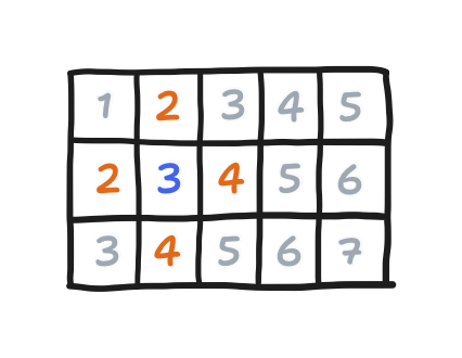
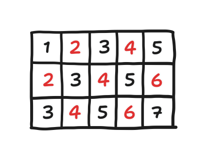
Finally, the difference between this and red-black Gauss-Seidel is this: by looping through the red points then through the black points, we’ve <em>permuted</em> the elements of $x$ (from the original $Ax = b$) into a new order that follows this looping, an order <em>distinct</em> from the conventional left-to-right bottom-to-top order, mapping from 2D position to 1D index. That’s best demonstrated with our good old three-by-three example.</p>

  <figure> 
<img src="/images/2024-09-26/figure15.png" alt="Two images made by filling in, with different colors, the lower-triangular (labeled as bottom and left), upper-triangular (labeled top and right), and diagonal (labeled center) parts of the given matrix A. On the left, one created from the three-by-three example. On the right, one created from the equivalent matrix on an input that was permuted in black-then-red order." />
<figcaption>

The color representation of $A$ from before, and a color representation of the equivalent matrix for an $x$ that was permuted in black-then-red order. (Fun fact: the three components can now be isolated by partitioning the matrix into a block matrix.)

</figcaption>
</figure>

  <p>Feel free to notice here how all the red points and black points are consecutive now!</p>

  <p>
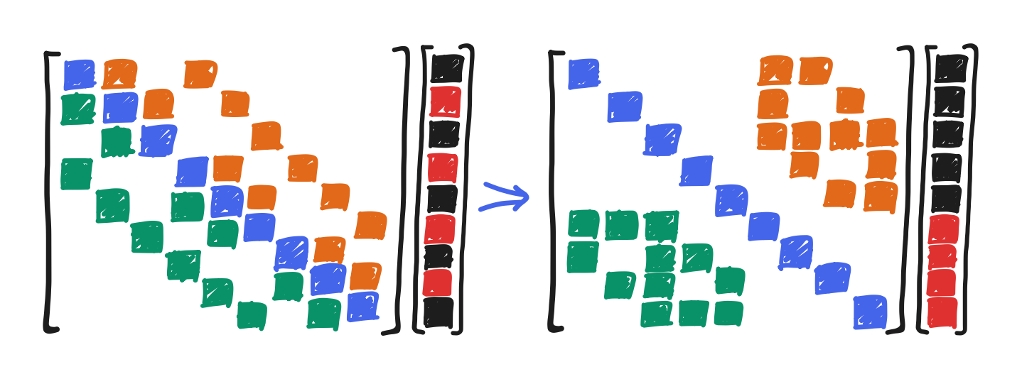
Formally, this can be written as a matrix similarity between $A$ and what we’ll call $A_\text{red-black}$, with a permutation matrix $P$ as the change-of-basis.</p>

\[P^{-1} A_\text{red-black} P = A\]

  <p>Then, $Ax = b$ can be written as $P^{-1} A_\text{red-black} P x = b$. This expresses how the elements of $x$ are permuted, put through $A_\text{red-black}$, then permuted back into conventional order. In practice, the red-black code doesn’t actually shuffle the memory. Rather, the changed looping does the work, like how the Gauss-Seidel code doesn’t actually do any substitutions to implement forward substitution.</p>

  <p>That said, though this matrix is definitionally similar, its $D + L + U$ splitting takes on a starkly different meaning. No longer does $L$ mean the left and bottom neighbors and $U$ mean the top and right neighbors. What <em>does</em> still stand is the fact that $L$ stands for the preceding and $U$ stands for the succeeding. Consider how $x$ is all-red and then all-black. Constructing a Gauss-Seidel procedure with this order gives the all-red-then-all-black looping. And in this procedure, $L$ comes to mean the red points and $U$ comes to mean the black points.</p>

</div>

<p>Last but not least, the next step beyond Gauss-Seidel iteration is “successive over-relaxation”, or “SOR”. The intuition of it goes like this: if stepping from $p^{(k)}[i, j]$ to $p^{(k+1)}[i, j]$ is in the right direction, what if we went <em>further</em> in that direction? It’s a linear extrapolation from $p^{(k)}[i, j]$ to $p^{(k+1)}[i, j]$ and onward. That is,</p>

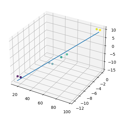
\[p_\text{SOR}^{(k+1)}[i, j] = \omega p_\text{G-S}^{(k+1)}[i, j] + (1-\omega) p^{(k)}[i, j]\]

<p>where $p_\text{G-S}^{(k+1)}[i, j]$ is the result from Gauss-Seidel iteration and $\omega$ is ordinarily a parameter between $0$ and $1$ that slides us between $p_\text{G-S}^{(k+1)}[i, j]$ and $p^{(k)}[i, j]$. It quite literally is the same expression as linear <em>interpolation</em> (yes, that lerp). But here, we’re free to push $\omega$ beyond $1$. Doing so can get us closer to the solution faster—much faster. Let’s look at its spectral radius.</p>

<p>So far, we have had nothing concrete to say about the spectral radius of Gauss-Seidel iteration—not what we can expect it to be, much less whether it is better than Jacobi iteration. The same can be said for SOR. To preface a bit first, you may have already realized that Gauss-Seidel can also be thought of as the $\omega = 1$ case of SOR. This means that an analysis of SOR will also cover Gauss-Seidel. That out of the way, Young found that, for matrices satisfying Property A, the spectral radius of SOR is a function of $\omega$ and the spectral radius of Jacobi iteration! Denoting $\rho(C_\text{Jac})$ as $\mu$ here, it goes like this:</p>

\[\rho(C_\omega) = \begin{cases} \frac{1}{4} \left( \omega \mu + \sqrt{\omega^2\mu^2 - 4(\omega-1)} \right)^2 &amp; 0 \leq \omega \leq \omega_\text{opt} \\ \omega - 1 &amp; \omega_\text{opt} \leq \omega \leq 2 \end{cases}\]

<p>where $\omega_\text{opt}$ is given by the following expression</p>

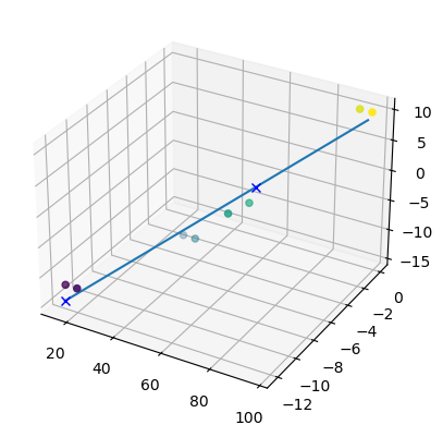
\[1 + \left( \frac{\mu}{1+\sqrt{1-\mu^2}} \right)^2\]

<p>and happens to be the value of $\omega$ that minimizes $\rho(C_\omega)$. The following plot make things clearer.</p>

<figure> 
<img src="/images/2024-09-26/figure16.svg" alt="Plots of the spectral radius of SOR iteration over the omega parameter, each one for a different spectral radius of Jacobi iteration. For any particular Jacobi radius, SOR radius decreases at accelerating speed until it reaches some minimum point, and from there it abrupt switches to rising linearly toward an endpoint of one (omega there being equal to two). The plots also show that, if the Jacobi radius lower, the corresponding SOR radius is lower." />
<figcaption>

Plots of a couple $\rho(C_\omega)$ curves, varying in $\mu$. It's continuous at $\omega_\text{opt}$, even though the definition is piecewise. By <a href="https://commons.wikimedia.org/wiki/File:Spectral_Radius.svg">HerrHartmuth via Wikimedia</a> and modified by me (adjusted the text). Hereby released under <a href="https://creativecommons.org/licenses/by-sa/4.0/deed.en">Creative Commons Attribution Share-Alike 4.0</a>.

</figcaption>
</figure>

<p>With this, we can check out what the radius of Gauss-Seidel iteration is. Plugging $1$ into the formula, we get that</p>

\[\begin{align*}\rho(C_1) &amp; = \frac{1}{4} \left( \mu + \sqrt{\mu^2} \right)^2 \\ &amp; = \frac{1}{4} (2\mu)^2 \\ &amp; = \mu^2 \end{align*}\]

<p>meaning that one Gauss-Seidel step is worth two Jacobi steps.</p>

<p>Now, let’s see how many Jacobi steps one SOR step is worth. Given our $60 \times 80$ grid and $\Delta x = 1$, we found earlier that our spectral radius was $0.9996$. Letting $\mu = 0.9996$, we get that $\omega_\text{opt} = 1.96$. Passing this into the formula for $\rho(C_\omega)$, we get that $\rho(C_{1.96}) = 0.96$. The number of steps is the exponent that takes $0.9996$ to $0.96$, or in other words $\log_{0.9996}(0.96) = 102.034$. One step of SOR is worth <em>over a hundred</em> Jacobi steps. Granted, at this point, I’d bet that we here have pushed the ideas of SOR to their breaking point. Here, I suspect that the <a href="https://en.wikipedia.org/wiki/Conjugate_gradient_method">“conjugate gradient”</a> method makes more sense. In fact, in that response I got from Stam, he mentioned that it was what he used to find the pressure, along with using a MAC grid. Though the grids aren’t the same, it sounds like it could work, but that must be a side project for another day. This has been a long post, and this has been a long series.</p>

<div class="note-panel">

  <p>This series has had more than a few tangents, and this one will be the last. I had seen the red-black order’s output looked much better than going in conventional order, so why did I assert that their spectral radii are the same?
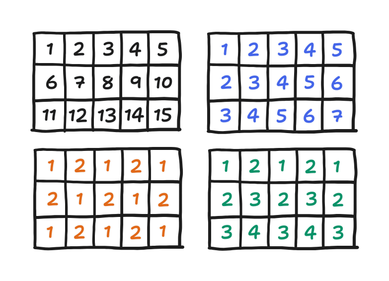
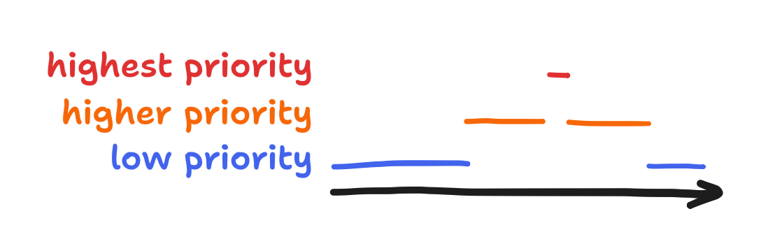
</p>

  <p>First, actually, <em>the order matters</em> in Young’s derivation of SOR’s spectral radius. It only holds if the order is what he called a “consistent order”. After going through what makes a “consistent order”, he went on to show four cases. Red-black is in indeed one of them, but the conventional order is <em>also</em> one. To list them all, there is</p>

  <ul>
    <li>$\sigma_1$, a left-to-right, top-to-bottom order (equivalent to left-to-right, bottom-to-top),</li>
    <li>$\sigma_2$, a wavefront order,</li>
    <li>$\sigma_3$, the red-black order, and</li>
    <li>$\sigma_4$, a zigzag order.</li>
  </ul>

  <p>You can see those orderings below. Points are in the order given by their numbers, though points with the same number can be evaluated in any order.</p>

  <figure> 
<img src="/images/2024-09-26/figure17.png" alt="Four grids of three-by-five, numbered in different orders. In the upper left, the numbering is increasing in left-to-right, top-to-bottom order. In the upper-right, the numbering starts at the top left then propogates down and to the right. In the bottom-left, the numbering is one or two in a checkerboard pattern i.e. red-black order. In the bottom-right, zigzags going from left to right while alternating between a row and its preceding row such that one can stack on top of another." />
<figcaption>

The four orderings Young described, all "consistent".

</figcaption>
</figure>

  <p>
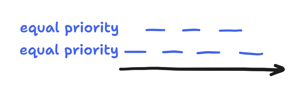
Because order doesn’t matter in Jacobi iteration, all orderings lead to the same $\rho(C_\text{Jacobi})$. Now, for a consistent order, $\rho(C_\omega)$ is a function of $\rho(C_\text{Jacobi})$. If the latter is the same, then so should be the former.</p>

  <p>Yet they look different when I actually run the two. Perhaps they have different eigenvectors? I don’t know why that is, really, but I went ahead and picked red-black SOR because there was no arguing against the fact that it looked better.</p>

</div>

<p>Here’s the culminating piece, a red-black SOR code, the thing that made ESP32-fluid-simulation possible.</p>

<div class="language-c highlighter-rouge"><div class="highlight"><pre class="highlight"><code><span class="k">struct</span> <span class="n">pois_context</span> <span class="p">{</span>
    <span class="kt">float</span> <span class="o">*</span><span class="n">d</span><span class="p">;</span>
    <span class="kt">float</span> <span class="n">dx</span><span class="p">;</span>
    <span class="kt">float</span> <span class="n">omega</span><span class="p">;</span>
<span class="p">};</span>

<span class="k">static</span> <span class="kt">float</span> <span class="nf">pois_sor_safe</span><span class="p">(</span><span class="kt">float</span> <span class="o">*</span><span class="n">p</span><span class="p">,</span> <span class="kt">int</span> <span class="n">i</span><span class="p">,</span> <span class="kt">int</span> <span class="n">j</span><span class="p">,</span> <span class="kt">int</span> <span class="n">dim_x</span><span class="p">,</span> <span class="kt">int</span> <span class="n">dim_y</span><span class="p">,</span>
        <span class="kt">void</span> <span class="o">*</span><span class="n">ctx</span><span class="p">)</span>
<span class="p">{</span>
    <span class="k">struct</span> <span class="n">pois_context</span> <span class="o">*</span><span class="n">pois_ctx</span> <span class="o">=</span> <span class="p">(</span><span class="k">struct</span> <span class="n">pois_context</span><span class="o">*</span><span class="p">)</span><span class="n">ctx</span><span class="p">;</span>
    <span class="kt">float</span> <span class="n">omega</span> <span class="o">=</span> <span class="n">pois_ctx</span><span class="o">-&gt;</span><span class="n">omega</span><span class="p">;</span>
    <span class="kt">float</span> <span class="n">p_gs</span> <span class="o">=</span> <span class="n">pois_expr_safe</span><span class="p">(</span><span class="n">p</span><span class="p">,</span> <span class="n">i</span><span class="p">,</span> <span class="n">j</span><span class="p">,</span> <span class="n">dim_x</span><span class="p">,</span> <span class="n">dim_y</span><span class="p">,</span> <span class="n">ctx</span><span class="p">);</span>
    <span class="k">return</span> <span class="p">(</span><span class="mi">1</span><span class="o">-</span><span class="n">omega</span><span class="p">)</span><span class="o">*</span><span class="p">(</span><span class="o">*</span><span class="n">p</span><span class="p">)</span> <span class="o">+</span> <span class="n">omega</span><span class="o">*</span><span class="n">p_gs</span><span class="p">;</span>
<span class="p">}</span>

<span class="k">static</span> <span class="kt">float</span> <span class="nf">pois_sor_fast</span><span class="p">(</span><span class="kt">float</span> <span class="o">*</span><span class="n">p</span><span class="p">,</span> <span class="kt">int</span> <span class="n">i</span><span class="p">,</span> <span class="kt">int</span> <span class="n">j</span><span class="p">,</span> <span class="kt">int</span> <span class="n">dim_x</span><span class="p">,</span> <span class="kt">int</span> <span class="n">dim_y</span><span class="p">,</span>
        <span class="kt">void</span> <span class="o">*</span><span class="n">ctx</span><span class="p">)</span>
<span class="p">{</span>
    <span class="k">struct</span> <span class="n">pois_context</span> <span class="o">*</span><span class="n">pois_ctx</span> <span class="o">=</span> <span class="p">(</span><span class="k">struct</span> <span class="n">pois_context</span><span class="o">*</span><span class="p">)</span><span class="n">ctx</span><span class="p">;</span>
    <span class="kt">float</span> <span class="n">omega</span> <span class="o">=</span> <span class="n">pois_ctx</span><span class="o">-&gt;</span><span class="n">omega</span><span class="p">;</span>

    <span class="kt">float</span> <span class="n">p_sum</span> <span class="o">=</span> <span class="p">(</span><span class="o">*</span><span class="p">(</span><span class="n">p</span><span class="o">-</span><span class="mi">1</span><span class="p">)</span> <span class="o">+</span> <span class="o">*</span><span class="p">(</span><span class="n">p</span><span class="o">+</span><span class="mi">1</span><span class="p">))</span> <span class="o">+</span> <span class="p">(</span><span class="o">*</span><span class="p">(</span><span class="n">p</span><span class="o">-</span><span class="n">dim_x</span><span class="p">)</span> <span class="o">+</span> <span class="o">*</span><span class="p">(</span><span class="n">p</span><span class="o">+</span><span class="n">dim_x</span><span class="p">));</span>

    <span class="kt">int</span> <span class="n">ij</span> <span class="o">=</span> <span class="n">index</span><span class="p">(</span><span class="n">i</span><span class="p">,</span> <span class="n">j</span><span class="p">,</span> <span class="n">dim_x</span><span class="p">);</span>
    <span class="kt">float</span> <span class="n">p_gs</span> <span class="o">=</span> <span class="o">-</span><span class="mi">0</span><span class="p">.</span><span class="mi">25</span><span class="n">f</span> <span class="o">*</span> <span class="p">(</span><span class="n">pois_ctx</span><span class="o">-&gt;</span><span class="n">dx</span> <span class="o">*</span> <span class="n">pois_ctx</span><span class="o">-&gt;</span><span class="n">d</span><span class="p">[</span><span class="n">ij</span><span class="p">]</span> <span class="o">-</span> <span class="n">p_sum</span><span class="p">);</span>

    <span class="k">return</span> <span class="p">(</span><span class="mi">1</span><span class="o">-</span><span class="n">omega</span><span class="p">)</span><span class="o">*</span><span class="p">(</span><span class="o">*</span><span class="n">p</span><span class="p">)</span> <span class="o">+</span> <span class="n">omega</span><span class="o">*</span><span class="n">p_gs</span><span class="p">;</span>
<span class="p">}</span>

<span class="kt">void</span> <span class="nf">poisson_solve</span><span class="p">(</span><span class="kt">float</span> <span class="o">*</span><span class="n">p</span><span class="p">,</span> <span class="kt">float</span> <span class="o">*</span><span class="n">div</span><span class="p">,</span> <span class="kt">int</span> <span class="n">dim_x</span><span class="p">,</span> <span class="kt">int</span> <span class="n">dim_y</span><span class="p">,</span> <span class="kt">float</span> <span class="n">dx</span><span class="p">,</span>
        <span class="kt">int</span> <span class="n">iters</span><span class="p">,</span> <span class="kt">float</span> <span class="n">omega</span><span class="p">)</span>
<span class="p">{</span>
    <span class="k">for</span> <span class="p">(</span><span class="kt">int</span> <span class="n">ij</span> <span class="o">=</span> <span class="mi">0</span><span class="p">;</span> <span class="n">ij</span> <span class="o">&lt;</span> <span class="n">dim_x</span><span class="o">*</span><span class="n">dim_y</span><span class="p">;</span> <span class="n">ij</span><span class="o">++</span><span class="p">)</span> <span class="p">{</span>
        <span class="n">p</span><span class="p">[</span><span class="n">ij</span><span class="p">]</span> <span class="o">=</span> <span class="mi">0</span><span class="p">;</span>
    <span class="p">}</span>
    <span class="k">struct</span> <span class="n">pois_context</span> <span class="n">pois_ctx</span> <span class="o">=</span> <span class="p">{.</span><span class="n">d</span> <span class="o">=</span> <span class="n">div</span><span class="p">,</span> <span class="p">.</span><span class="n">dx</span> <span class="o">=</span> <span class="n">dx</span><span class="p">,</span> <span class="p">.</span><span class="n">omega</span> <span class="o">=</span> <span class="n">omega</span><span class="p">};</span>
    <span class="k">for</span> <span class="p">(</span><span class="kt">int</span> <span class="n">k</span> <span class="o">=</span> <span class="mi">0</span><span class="p">;</span> <span class="n">k</span> <span class="o">&lt;</span> <span class="n">iters</span><span class="p">;</span> <span class="n">k</span><span class="o">++</span><span class="p">)</span> <span class="p">{</span>
        <span class="n">domain_iter_red_black</span><span class="p">(</span><span class="n">pois_sor_safe</span><span class="p">,</span> <span class="n">pois_sor_fast</span><span class="p">,</span> <span class="n">p</span><span class="p">,</span> <span class="n">p</span><span class="p">,</span> <span class="n">dim_x</span><span class="p">,</span> <span class="n">dim_y</span><span class="p">,</span>
            <span class="o">&amp;</span><span class="n">pois_ctx</span><span class="p">);</span>
    <span class="p">}</span>
<span class="p">}</span>
</code></pre></div></div>

<p>
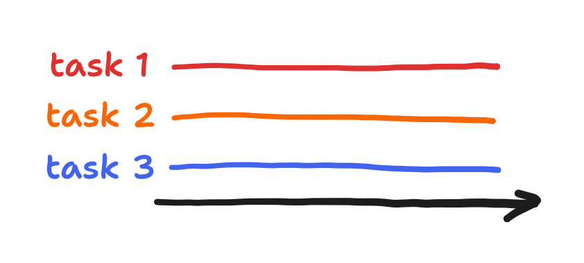
In summary, to compute a divergence-free velocity field, we applied the Helmholtz-Hodge decomposition, but the decomposition itself gave us a boundary value problem to solve. Through discretization, we turned that problem into a massive $Ax = b$ problem, but one where $A$ was sparse. We used that sparsity to our advantage, choosing to approximately solve it with an iterative method that lets us compute the next guess at $x$ one element at a time—skipping the zeroes along the way. The first one we saw was Jacobi iteration. I shared how I got its spectral radius. Then, we saw Gauss-Seidel iteration and SOR. Finally, we learned that, for the class of matrices satisfying Property A, including our $A$, Gauss-Seidel was faster and SOR was dramatically faster. All this context was necessary to figuring out how to run a fluid sim on an ESP32.</p>

<p>
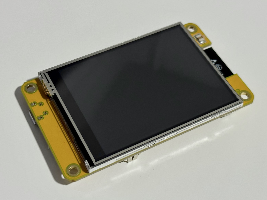
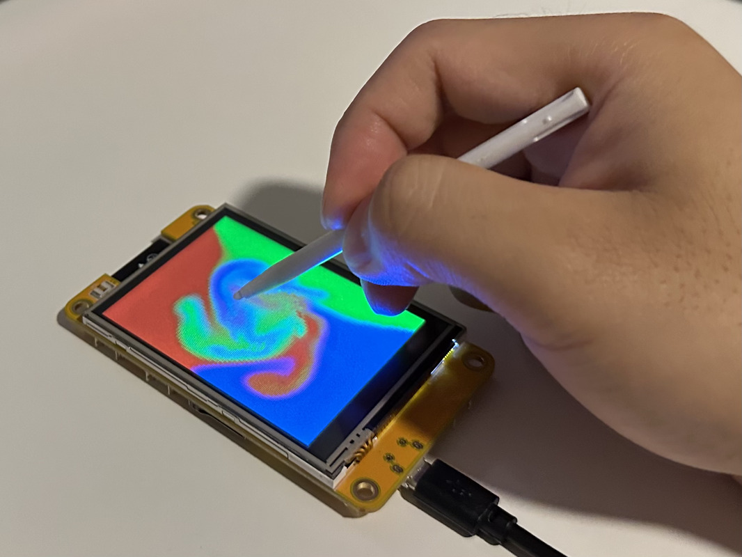
With that, the actual fluid sim mechanism in ESP32-fluid-simulation is entirely covered, and that caps off the tour through its use of FreeRTOS, the Cheap Yellow Display (CYD), and the Navier-Stokes equations. This was quite the epic undertaking for me, building the sim more than one year ago then going to write on and off about it since. I’d do it again, considering that—in trying to explain it—I ended up formalizing my own understanding of my own project and updated it accordingly along the way. And now that understanding is here on the internet.</p>

<p>That said, this project is far from the last one I’ll ever make then write about. Look out for the next series, to be announced some day. In any case and for the last time, you can see <a href="https://github.com/colonelwatch/ESP32-fluid-simulation">ESP32-fluid-simulation</a> on GitHub!</p>]]></content><author><name>Kenny Peng</name><email>kenny@kennypeng.com</email></author><summary type="html"><![CDATA[It’s been a while since my last post, but let’s bring this series to its finale. Out of all the parts of the fluid sim, the last piece I have not explained is the pressure projection. The code alone doesn’t reveal the great deal of context that goes into its design. Here’s a hint: it’s actually a linear algebra routine involving a “sparse matrix”. Though it’s possible these days to implement the pressure projection without needing to know all that context, thanks to articles like Jamie Wong’s post, the GPU Gems chapter, and Stam’s “Real-Time Fluid Dynamics for Games”, achieving a believable fluid simulation on an ESP32 would have been impossible. I’ve personally tried it before, and after knowing? All I needed was to switch in a technically superior method. There was a reason why I dedicated airtime to this—let me explain.]]></summary></entry><entry><title type="html">Rebuilding ESP32-fluid-simulation: the advection and force steps of the sim task (Part 4)</title><link href="http://kennypeng.com/2024/01/20/esp32_fluid_sim_4.html" rel="alternate" type="text/html" title="Rebuilding ESP32-fluid-simulation: the advection and force steps of the sim task (Part 4)" /><published>2024-01-20T00:00:00+00:00</published><updated>2024-01-20T00:00:00+00:00</updated><id>http://kennypeng.com/2024/01/20/esp32_fluid_sim_4</id><content type="html" xml:base="http://kennypeng.com/2024/01/20/esp32_fluid_sim_4.html"><![CDATA[<p>If you’ve read <a href="/2023/07/30/esp32_fluid_sim_2.html">Part 2</a> and <a href="/2023/09/22/esp32_fluid_sim_3.html">Part 3</a> already, then you’re as equipped to read this part as I can make you. You would have already heard me mention that we should be passing in touch inputs, consisting of locations of velocities. You also would have already heard that we’re getting out color arrays. Some mechanism should be turning the former into the latter, and it should be broadly inspired by the physics, which is written out as partial differential equations. This post and the next post—the final ones—are about that mechanism. To be precise, this post covers everything but the pressure step, and the next will give that step its own airtime.</p>

<p>With that said, if I miss anything, the references I used might be helpful. That’s the <a href="https://developer.nvidia.com/gpugems/gpugems/part-vi-beyond-triangles/chapter-38-fast-fluid-dynamics-simulation-gpu">GPU Gems chapter</a> and <a href="https://jamie-wong.com/2016/08/05/webgl-fluid-simulation/">Jamie Wong’s blog post</a>, but there’s also Stam’s <a href="https://damassets.autodesk.net/content/dam/autodesk/www/autodesk-reasearch/Publications/pdf/realtime-fluid-dynamics-for.pdf">“Real-time Fluid Dynamics for Games”</a> and <a href="https://dl.acm.org/doi/pdf/10.1145/311535.311548">“Stable Fluids”</a>.</p>

<p>Now, to tell you what I’m going to tell you, a high-level overview is this:</p>

<ol>
  <li>apply “semi-Lagrangian advection”, an implementation of the advection operator (for “advection”, see Part 3), to the velocities,</li>
  <li>apply the user’s input to the velocities,</li>
  <li>apply “divergence-free projection” to velocities in order to correct it (i.e. the pressure step briefed in Part 3 and to be explained in the next part) and finally,</li>
  <li>apply semi-Lagrangian advection to the density array with the updated velocities.</li>
</ol>

<p>The process has four parts, and each part corresponds to a part of the physics. Let’s recall the partial differential equations that we ended up with in Part 3, that is:</p>

\[\frac{\partial \rho}{\partial t} = - (\bold v \cdot \nabla) \rho\]

\[\frac{\partial \bold v}{\partial t} = - (\bold v \cdot \nabla) \bold v - \frac{1}{\rho} \nabla p + \bold f\]

\[\nabla \cdot \bold v = 0\]

<p>Setting aside the incompressibility constraint for now—that’s the third equation $\nabla \cdot \bold v = 0$—the equations can be split into four terms. That’s one term for each part of the process. To list them in the order of their corresponding steps, there’s the advection of the velocity $-(\bold v \cdot \nabla) \bold v$, the applied force $\bold f$, the pressure $- \frac{1}{\rho} \nabla p$, and the advection of the density $-(\bold v \cdot \nabla) \rho$.</p>

<p>Before we get into each term and its corresponding part of the process, there’s a key piece of context to keep in mind. We’re faced with the definitions of $\frac{\partial \rho}{\partial t}$ and $\frac{\partial \bold v}{\partial t}$ here, and they have solutions which are density and velocity fields that evolve over time. That’s not computable. Computers can’t operate on fields—the functions of continuous space that they are—much less operate on ones that continuously vary over time. Instead, time and space need to be “discretized”.</p>

<p>Let’s tackle the discretization of time first. Continuous time can be approximated by a <em>sequence</em> of closely-spaced points in time. Usually, those points in time are regularly spaced apart by a timestep $\Delta t$, In other words, we use the sequence $\{\; 0,\; \Delta t,\; 2 \Delta t,\; 3 \Delta t,\; \dots \;\}$. The result should be that a field at some time $t$ in the sequence can be approximately expressed in terms of the field at the <em>previous</em> time $t_0 - \Delta t$. That is, we should be able to calculate an <em>update</em> to the fields. You may see how this is useful for running simulations. This general idea is called “numerical integration”, the simplest case being <a href="https://en.wikipedia.org/wiki/Euler_method">Euler’s method</a>—yes, that Euler’s method, if you still remember it. In other cases, methods like <a href="https://en.wikipedia.org/wiki/Backward_Euler_method">implicit Euler</a>, <a href="https://en.wikipedia.org/wiki/Runge%E2%80%93Kutta_methods">Runge-Kutta</a>, and <a href="https://en.wikipedia.org/wiki/Leapfrog_integration">leapfrog integration</a> offer better accuracy and/or stability, but that’s out-of-scope.</p>

<p>Now, let’s tackle the discretization of space. Continuous space can be approximated by a mesh of points, each point being associated with the value of the field there. In the simplest case, that mesh is a regular grid. Also remember that fields are functions of location. Combining these two things, we get the incredibly convenient conclusion that discretized fields can be expressed as an <em>array of values</em>. For each index into the array $(i, j)$, there is a corresponding point on the grid $(x_i, y_j)$, and for every point, there is a value of the field at that point. If we wanted to initialize an array from some known field, we could just evaluate the field on each point of the grid and then assign the value to the associated cell of the array.</p>

<figure>
<img src="/images/2024-01-20/figure1.png" alt="On the left, a surface plot of x squared plus y squared, and on the right a grid filled with numbers, namely the values of x squared plus y squared at integer values of x and y" />
<figcaption>

Using discretization with a grid, an array of the field's values can stand for the field itself. Grids are defined by their grid lengths $\Delta x$ and $\Delta y$. In this example, $\Delta x = \Delta y = 1$ is a special case where the field is evaluated at integer values of $x$ and $y$.

</figcaption>
</figure>

<div class="note-panel">

  <p>Side note: it’s a fair question to ask here why $(i, j)$ doesn’t correspond to—say—$(x_j, y_i)$ instead. Why does $i$ select the horizontal component and not the vertical one? This continues from my tangent about indexing in Part 2. The answer is that you <em>could</em> go about it that way and then derive a different but entirely consistent discretization. In fact, I originally had it that way. However, I switched out of that to keep all the expressions looking like how they do in the literature. So, in short, the reason is just convention.</p>

  <p>Second side note: this is not to say that the array is a <em>matrix</em>. The array is only two-dimensional because the space is two-dimensional. If the space was three-dimensional, then so would be the array. And forget about arrays if the mesh isn’t a grid! So, most matrix operations wouldn’t mean anything either. It’d be more correct to think of discretized fields as very long vectors, but we’re encroaching on a next-post matter now.</p>

</div>
<p><!-- div class="note-panel" --></p>

<p>A grid discretization is what Stam went with, and for that reason, it’s what’s used here.</p>

<p>A key result of discretizing space is that the differential operators can be approximated by differences (i.e. subtraction) between the values of the field at a point and its neighbors. In particular, using a grid can make the partial derivatives into something incredibly simple: $\frac{\partial}{\partial x}$ into the value of the right neighbor minus the value of the left neighbor and $\frac{\partial}{\partial y}$ into the top minus the bottom. But that’s getting into “finite difference methods”, of which the pressure step is one such method. We’ll get to that in the next post. For now, it’s enough to say that, in general, discretizing with a grid is the simple choice for making computers operate on fields.</p>

<p>With that said, we’ll soon see that “semi-Lagrangian advection” does something unique with the grid.</p>

<p>To sum up this “just for context” moment, to compute an approximate solution to the presented partial differential equations, we need two levels of discretization. First, we need to discretize time, turning it into a scheme of updating the density and velocity fields repeatedly. Then, we need to discretize space to make the update computable. And so, time is replaced with a sequence, and space is replaced with a grid. All this is because computers cannot handle functions of continuous time nor functions of continuous space, let alone functions of both like an evolving field. Now, all this is quite abstract, and that’s because each part invokes the discretization of time and space <em>slightly differently</em>, and we’ll go into the details of each.</p>

<p>With all that said, in the face of our definitions of $\frac{\partial \rho}{\partial t}$ and $\frac{\partial \bold v}{\partial t}$, this generally means that the density/concentration field (which I’m currently just calling the density field out of expediency) and the velocity field become just density and velocity arrays, and we should be able to calculate their updates. In this situation, we can update the arrays in accordance with the partial differential equations by going <em>term by term</em>, hence why each step of the overall process corresponds to a single term. (Though, I’m not sure if the implicit assumption of independence between the terms that underlies going term by term is just an expedient approximation or our math-given right. Anyway…) Let’s go over the four parts, step by step.</p>

<p>The first step is the “semi-Lagrangian advection” of the velocities, implementing the $-(\bold v \cdot \nabla) \bold v$ term. A key highlight here: Stam’s treatment of the advection term is <em>not</em> a finite difference method, yet it still uses discretization with a grid! I’d also like to highlight a bit of how Stam arrived at this method. All that information is largely documented between “Stable Fluids” and “Real-Time Fluid Dynamics for Games”.</p>

<p>In “Stable Fluids”, there is a formal analysis that involves a technique called a “method of characteristics”. It’s a whole proof, but a sketch of it is this: at every point $\bold x$ (that’s the coordinate vector $\bold x$, as covered in Part 2), there is a particle, and that particle arrived there from somewhere. Let $\bold{p}(\bold x, t)$ be its path, such that the current location is defined by the equality $\bold{p}(\bold x, t_0) = \bold x$ where $t_0$ is the current time. Then, $\bold{p}(\bold x, t_0 - \Delta t)$ is where the particle was in the previous time.</p>

<figure>
<img src="/images/2024-01-20/figure2.png" alt="In orange, a velocity field as a vector plot. In blue, a path of a particle that follows the velocity field. In black, a point on the path that represents the position of the particle at time t_0. In grey, a point on the path that represents where the particle was previously at time t_0 minus Delta t." />
<figcaption>

Given some velocity field, the path of a particle and its locations at time $t_0$ and $t_0 - \Delta t$

</figcaption>
</figure>

<p>As a result, the particle must have carried its properties along the way, and one of them is said to be momentum, or in other words, velocity. Therefore, an advection update looks like the assignment of the field value at the previous location, $\bold{p}(\bold x, t_0 - \Delta t)$, to the field at the current location, $\bold x$. This is the result of Stam’s analysis, and it can be written as the following:</p>

\[\bold{v}_\text{advect}(\bold x) = \bold{v}(\bold{p}(\bold x, t_0 - \Delta t))\]

<p>There is a unique time discretization here, but we’re not done yet! It’s still not computable because it’s missing a discretization of space. Of course, Stam presented one in “Stable Fluids” too. The calculation of $\bold{v}_\text{advect}$ can be done at just the points on the grid, and for each point, a “Runge-Kutta back-tracing” on the velocity field can be used to find $\bold{p}(\bold x, t_0 - \Delta t)$.</p>

<p>I won’t get into how that works, and I won’t have to in a moment. We’re one further approximation away from the method that appears in “Real-time Fluid Dynamics for Games” (and also the GPU Gems article and Wong’s post). Quite simply, if finding the path from $\bold{p}(\bold x, t_0 - \Delta t)$ to $\bold x$ can be called a “nonlinear” backtracing, then it’s replaced with a <em>linear</em> backtracing. The path is approximated with a straight line that extends from $\bold x$ in the direction of the velocity there:</p>

\[\bold{v}_\text{advect}(x) = \bold{v}(\bold x - \bold{v}(\bold x) \Delta t, t)\]

<p>or in other words $\bold x - \bold{v}(\bold x) \Delta t$ replaces $\bold{p}(\bold x, t - \Delta t)$</p>

<figure>
<img src="/images/2024-01-20/figure6.png" alt="In orange, a velocity field as a vector plot. In blue, a straight line that approximates a path of a particle that follows the vector field and extends in the direction of the velocity. In black, a point on the path that represents the position of the particle at time t_0, specifically a particle at a point that coincides on the grid of arrows i.e. the vector plot. In grey, an approximation of the point where the particle was previously at time t_0 - Delta t." />
</figure>

<p>This expression is usually shown on its own, but it’s really three parts: a “method of characteristics” analysis that comprises a time discretization, a space discretization using a grid, and a further approximation using a linear backtracing.</p>

<p>Anyway, the found point almost certainly doesn’t coincide with a point on the grid, so Stam dealt with this by <a href="https://en.wikipedia.org/wiki/Bilinear_interpolation#Application_in_image_processing">“bilinearly interpolating”</a> between the four closest velocity values.</p>

<figure>
<img src="/images/2024-01-20/figure3.png" alt="Four arrows on the corners of a square on the grid, each pointed in different directions. Dashed lines connect the top two arrows and the bottom two arrows. Points dot halfway on the dashed lines. On the top point, an arrow points in the direction of the top two arrows' average. On the bottom point, an arrow points the direction of the bottom two arrows' average. Another dashed line connects the points on the dashed line. Less than half-way on the dashed line, there is a point and an arrow that points in the weighted average of the arrows on the dashed lines, with more weight given to the top arrow." />
</figure>

<p>For more information on that, see the above link to Wikipedia. It’s got a better explanation of bilinear interpolation than one I can make—diagrams included. With that said, bilinear interpolation also amounts to very little code.</p>

<div class="language-c++ highlighter-rouge"><div class="highlight"><pre class="highlight"><code><span class="k">template</span><span class="o">&lt;</span><span class="k">typename</span> <span class="nc">T</span><span class="p">&gt;</span>
<span class="k">using</span> <span class="n">TPromoted</span> <span class="o">=</span> <span class="k">decltype</span><span class="p">(</span><span class="n">std</span><span class="o">::</span><span class="n">declval</span><span class="o">&lt;</span><span class="n">T</span><span class="o">&gt;</span><span class="p">()</span> <span class="o">*</span> <span class="n">std</span><span class="o">::</span><span class="n">declval</span><span class="o">&lt;</span><span class="kt">float</span><span class="o">&gt;</span><span class="p">());</span>

<span class="k">template</span> <span class="o">&lt;</span><span class="k">class</span> <span class="nc">T</span><span class="p">&gt;</span>
<span class="k">static</span> <span class="n">TPromoted</span><span class="o">&lt;</span><span class="n">T</span><span class="o">&gt;</span> <span class="n">lerp</span><span class="p">(</span><span class="kt">float</span> <span class="n">di</span><span class="p">,</span> <span class="n">T</span> <span class="n">p1</span><span class="p">,</span> <span class="n">T</span> <span class="n">p2</span><span class="p">)</span>
<span class="p">{</span>
    <span class="k">return</span> <span class="n">p1</span> <span class="o">*</span> <span class="p">(</span><span class="mi">1</span> <span class="o">-</span> <span class="n">di</span><span class="p">)</span> <span class="o">+</span> <span class="n">p2</span> <span class="o">*</span> <span class="n">di</span><span class="p">;</span>
<span class="p">}</span>

<span class="k">template</span> <span class="o">&lt;</span><span class="k">class</span> <span class="nc">T</span><span class="p">&gt;</span>
<span class="k">static</span> <span class="n">TPromoted</span><span class="o">&lt;</span><span class="n">T</span><span class="o">&gt;</span> <span class="n">billinear_interpolate</span><span class="p">(</span><span class="kt">float</span> <span class="n">di</span><span class="p">,</span> <span class="kt">float</span> <span class="n">dj</span><span class="p">,</span> <span class="n">T</span> <span class="n">p11</span><span class="p">,</span> <span class="n">T</span> <span class="n">p12</span><span class="p">,</span>
                                          <span class="n">T</span> <span class="n">p21</span><span class="p">,</span> <span class="n">T</span> <span class="n">p22</span><span class="p">)</span>
<span class="p">{</span>
    <span class="k">return</span> <span class="n">lerp</span><span class="p">(</span><span class="n">di</span><span class="p">,</span> <span class="n">lerp</span><span class="p">(</span><span class="n">dj</span><span class="p">,</span> <span class="n">p11</span><span class="p">,</span> <span class="n">p12</span><span class="p">),</span> <span class="n">lerp</span><span class="p">(</span><span class="n">dj</span><span class="p">,</span> <span class="n">p21</span><span class="p">,</span> <span class="n">p22</span><span class="p">));</span>
<span class="p">}</span>
</code></pre></div></div>

<p>For this project, which in C++, that code uses templates. That lets it handle multiple types, which it will see because—remember—there are <em>two</em> advection terms! There’s one for velocity <em>and</em> there’s one for density. Much of the work presented for velocity will be reused, via templates. And if you’re wondering about the <code class="language-plaintext highlighter-rouge">using TPromoted</code> expression. The simplest way to write linear interpolation is with floating-point, and once we’re in floating point, we may as well stay in floating point, only converting back at the very end. This includes floating-point vector classes, which is why <code class="language-plaintext highlighter-rouge">decltype</code> is used instead of just a <code class="language-plaintext highlighter-rouge">float</code> type.</p>

<p>With that in mind, it’s simply a matter of computing the source and getting the bilinear interpolation with that point. Here’s a sample of code from the project that does this.</p>

<div class="language-c++ highlighter-rouge"><div class="highlight"><pre class="highlight"><code><span class="k">template</span> <span class="o">&lt;</span><span class="k">class</span> <span class="nc">T</span><span class="p">&gt;</span>
<span class="k">static</span> <span class="n">T</span> <span class="nf">sample</span><span class="p">(</span><span class="n">T</span> <span class="o">*</span><span class="n">p</span><span class="p">,</span> <span class="kt">float</span> <span class="n">i</span><span class="p">,</span> <span class="kt">float</span> <span class="n">j</span><span class="p">,</span> <span class="kt">int</span> <span class="n">dim_x</span><span class="p">,</span> <span class="kt">int</span> <span class="n">dim_y</span><span class="p">,</span> <span class="kt">bool</span> <span class="n">no_slip</span><span class="p">)</span> <span class="p">{</span>
    <span class="kt">bool</span> <span class="n">x_under</span> <span class="o">=</span> <span class="n">i</span> <span class="o">&lt;</span> <span class="mi">0</span><span class="p">;</span>
    <span class="kt">bool</span> <span class="n">x_over</span> <span class="o">=</span> <span class="n">i</span> <span class="o">&gt;=</span> <span class="n">dim_x</span> <span class="o">-</span> <span class="mi">1</span><span class="p">;</span>
    <span class="kt">bool</span> <span class="n">y_under</span> <span class="o">=</span> <span class="n">j</span> <span class="o">&lt;</span> <span class="mi">0</span><span class="p">;</span>
    <span class="kt">bool</span> <span class="n">y_over</span> <span class="o">=</span> <span class="n">j</span> <span class="o">&gt;=</span> <span class="n">dim_y</span> <span class="o">-</span> <span class="mi">1</span><span class="p">;</span>

    <span class="kt">bool</span> <span class="n">x_oob</span> <span class="o">=</span> <span class="n">x_under</span> <span class="o">||</span> <span class="n">x_over</span><span class="p">;</span>
    <span class="kt">bool</span> <span class="n">y_oob</span> <span class="o">=</span> <span class="n">y_under</span> <span class="o">||</span> <span class="n">y_over</span><span class="p">;</span>

    <span class="kt">float</span> <span class="n">i_floor</span> <span class="o">=</span> <span class="n">floorf</span><span class="p">(</span><span class="n">i</span><span class="p">),</span> <span class="n">j_floor</span> <span class="o">=</span> <span class="n">floorf</span><span class="p">(</span><span class="n">j</span><span class="p">);</span>
    <span class="kt">float</span> <span class="n">di</span> <span class="o">=</span> <span class="n">i</span> <span class="o">-</span> <span class="n">i_floor</span><span class="p">,</span> <span class="n">dj</span> <span class="o">=</span> <span class="n">j</span> <span class="o">-</span> <span class="n">j_floor</span><span class="p">;</span>
    <span class="kt">int</span> <span class="n">ij</span><span class="p">;</span>

    <span class="k">if</span> <span class="p">(</span><span class="o">!</span><span class="n">x_oob</span> <span class="o">&amp;&amp;</span> <span class="o">!</span><span class="n">y_oob</span><span class="p">)</span> <span class="p">{</span>   <span class="c1">// typical case: not near the boundary</span>
        <span class="n">ij</span> <span class="o">=</span> <span class="n">index</span><span class="p">(</span><span class="n">i_floor</span><span class="p">,</span> <span class="n">j_floor</span><span class="p">,</span> <span class="n">dim_x</span><span class="p">);</span>
        <span class="k">return</span> <span class="n">billinear_interpolate</span><span class="p">(</span><span class="n">di</span><span class="p">,</span> <span class="n">dj</span><span class="p">,</span> <span class="n">p</span><span class="p">[</span><span class="n">ij</span><span class="p">],</span> <span class="n">p</span><span class="p">[</span><span class="n">ij</span> <span class="o">+</span> <span class="n">dim_x</span><span class="p">],</span> <span class="n">p</span><span class="p">[</span><span class="n">ij</span> <span class="o">+</span> <span class="mi">1</span><span class="p">],</span>
                                     <span class="n">p</span><span class="p">[</span><span class="n">ij</span> <span class="o">+</span> <span class="n">dim_x</span> <span class="o">+</span> <span class="mi">1</span><span class="p">]);</span>
    <span class="p">}</span>

    <span class="c1">// OMITTED</span>
<span class="p">}</span>

<span class="k">template</span> <span class="o">&lt;</span><span class="k">class</span> <span class="nc">T</span><span class="p">,</span> <span class="k">class</span> <span class="nc">U</span><span class="p">&gt;</span>
<span class="kt">void</span> <span class="n">advect</span><span class="p">(</span><span class="n">T</span> <span class="o">*</span><span class="n">next_p</span><span class="p">,</span> <span class="n">T</span> <span class="o">*</span><span class="n">p</span><span class="p">,</span> <span class="n">Vector2</span><span class="o">&lt;</span><span class="n">U</span><span class="o">&gt;</span> <span class="o">*</span><span class="n">vel</span><span class="p">,</span> <span class="kt">int</span> <span class="n">dim_x</span><span class="p">,</span> <span class="kt">int</span> <span class="n">dim_y</span><span class="p">,</span> <span class="kt">float</span> <span class="n">dt</span><span class="p">,</span>
            <span class="kt">bool</span> <span class="n">no_slip</span><span class="p">)</span>
<span class="p">{</span>
    <span class="k">for</span> <span class="p">(</span><span class="kt">int</span> <span class="n">i</span> <span class="o">=</span> <span class="mi">0</span><span class="p">;</span> <span class="n">i</span> <span class="o">&lt;</span> <span class="n">dim_x</span><span class="p">;</span> <span class="n">i</span><span class="o">++</span><span class="p">)</span> <span class="p">{</span>
        <span class="k">for</span> <span class="p">(</span><span class="kt">int</span> <span class="n">j</span> <span class="o">=</span> <span class="mi">0</span><span class="p">;</span> <span class="n">j</span> <span class="o">&lt;</span> <span class="n">dim_y</span><span class="p">;</span> <span class="n">j</span><span class="o">++</span><span class="p">)</span> <span class="p">{</span>
            <span class="kt">int</span> <span class="n">ij</span> <span class="o">=</span> <span class="n">index</span><span class="p">(</span><span class="n">i</span><span class="p">,</span> <span class="n">j</span><span class="p">,</span> <span class="n">dim_x</span><span class="p">);</span>
            <span class="n">Vector2</span><span class="o">&lt;</span><span class="kt">float</span><span class="o">&gt;</span> <span class="n">source</span> <span class="o">=</span> <span class="n">Vector2</span><span class="o">&lt;</span><span class="kt">float</span><span class="o">&gt;</span><span class="p">(</span><span class="n">i</span><span class="p">,</span> <span class="n">j</span><span class="p">)</span> <span class="o">-</span> <span class="n">vel</span><span class="p">[</span><span class="n">ij</span><span class="p">]</span> <span class="o">*</span> <span class="n">dt</span><span class="p">;</span>
            <span class="n">next_p</span><span class="p">[</span><span class="n">ij</span><span class="p">]</span> <span class="o">=</span> <span class="n">sample</span><span class="p">(</span><span class="n">p</span><span class="p">,</span> <span class="n">source</span><span class="p">.</span><span class="n">x</span><span class="p">,</span> <span class="n">source</span><span class="p">.</span><span class="n">y</span><span class="p">,</span> <span class="n">dim_x</span><span class="p">,</span> <span class="n">dim_y</span><span class="p">,</span> <span class="n">no_slip</span><span class="p">);</span>
        <span class="p">}</span>
    <span class="p">}</span>
<span class="p">}</span>
</code></pre></div></div>

<p>Here, the <code class="language-plaintext highlighter-rouge">advect</code> function loops over every point on the grid, calculating the source for each and assigning the result of the <code class="language-plaintext highlighter-rouge">sample</code> function. The <code class="language-plaintext highlighter-rouge">sample</code> function in turn calls the earlier given <code class="language-plaintext highlighter-rouge">bilinear_interpolate</code> function.</p>

<p>But I’ve omitted the rest of the <code class="language-plaintext highlighter-rouge">sample</code> function! Notice that it returns early if the source <em>is not</em> near the boundary. That creates a fast path, and that means the omitted code was for handling when it <em>is</em> near the boundary.</p>

<p>So, what have I hidden? I’ll answer with another question. What if the backtracing sends us to the boundary of the domain, or even beyond it?</p>

<p>It’s a fair question to ask, and it’s an important question because what we should do here directly depends on what the boundary is <em>physically</em>. In our case, the boundary is a solid wall. Here, I turn to the GPU Gems article, where it’s written that the “no-slip” condition hence applies, which just means the velocity there must be zero. Why the change again in my references? The “Stable Fluids” paper assumed a different physical condition, “periodic” boundaries that essentially imply a tile-able cell or a “toroidal” i.e. donut-shaped domain, but the “Real-time Fluid Dynamics for Games” paper chose a somewhat looser condition that was still based on solid walls. Between that and no-slip conditions, no-slip conditions are easier to build upon. For starters, a no-slip condition is more easily implemented inside a bilinear interpolation scheme—inside the <code class="language-plaintext highlighter-rouge">sample</code> function, that is.</p>

<p>For now, let’s focus on the bottom row. Below the bottom row, we can construct a ghost row that always takes the <em>negative</em> of its values. Therefore, any linear interpolation at the halfway point between the bottom row and the ghost row must be equal to zero. That is, the <em>halfway line</em> between them achieves the no-slip condition, thereby simulating the solid wall. From there, if the backtracing gives a position that is beyond the halfway line, it should just be clamped to it. Finally, this approach with the ghost row extends to all sides of the domain.</p>

<figure>
<img src="/images/2024-01-20/figure4.png" alt="In the background, the bottom half of the image is hashed out, signifying a solid wall. Four arrows are on the corners of a square on the grid, the top two pointed in different directions but the bottom two pointing in the opposite direction of the top two. Dashed lines connect the top two arrows and the bottom two arrows. Points dot halfway on the dashed lines. On the top point, an arrow points in the direction of the top two arrows' average. On the bottom point, an arrow points in the direction of the bottom twos' average, and notably this is also in the opposite direction of the arrow on the top point. Another dashed line connects the points on the dashed lines. A point dots halfway on this new line. On this new point, a smaller point dots on top of it, signifying that the average of the two averages, which are opposites of each other, is zero." />
<figcaption>

The ghost row exists <i>inside</i> the wall, and the value of the bilinear interpolation on the wall's surface must be zero

</figcaption>
</figure>

<p>We also need to define the value of the ghost corner formed by a ghost row and ghost column. I didn’t see a rigorous treatment of them in my references, and I’ve seen that the corners might not matter much in practice. Still, the “no-slip” condition has a nice internal consistency that just gives us this definition. At the intersection of the halfway lines, the velocity there must also be zero. From this, we can form <em>an equation involving the value of the ghost corner</em>, and its solution is that the ghost corner should take on the value of the real corner—<em>not</em> its negative! Rather, it can be thought of as the ghost row taking the negative of the value at the end of the ghost column, which is itself a negative, and so making a double negative.</p>

<figure>
<img src="/images/2024-01-20/figure5.png" alt="In the background, the left half and bottom half of the image is hashed out, signifying intersecting solid walls. Four arrows are on the corners of a square on the grid. The upper right arrow is pointed in some direction, the upper left and bottom right is pointed in the opposite direction, and the bottom left arrow is pointed in the same direction. Dashed lines connect the top two arrows and the bottom two arrows. Points dot halfway on the dashed lines. On each of the two points is a smaller point, signifying that the average of the top two arrows and the average of the bottom two arrows is both zero. Another dashed line connects the points on the dashed lines. A point dots halfway on this new line. On this point, a smaller point dots on top of it, signifying that the average of the two averages, which are themselves zero, is zero." />
</figure>

<p>That said, the project doesn’t actually handle the boundary with ghost rows/columns, which is how it’s done in “Real-time Fluid Dynamics for Games” and the GPU Gems article. It used to, but now it uses something different but equivalent. To understand the difference, it is important to recognize that the negative values are just constructs on the way to defining the halfway line, where the no-slip condition is enforced and beyond which no source point is supposed to exist.</p>

<p>Let’s now draw the bilinear interpolation as a 3D surface. The construction of the halfway line ends up looking like this.</p>

<figure>
<img src="/images/2024-01-20/figure7.png" alt="diagram of surface created by bilinear interpolation at a domain corner, showing a no-slip condition being implicitly enforced by ghost points and negative velocity values" />
<figcaption>

Dashed lines are obscured or purely virtual constructions.

</figcaption>
</figure>

<p>The ghost rows and columns take on negative values, and so the surface does indeed flip in sign as it crosses the halfway line. As mentioned before though, source points are to never cross that line, and they’re to be clamped to it if they do. As a result, the <em>samples</em> of that surface will <em>never</em> flip in sign. In that sense, the negative values are just virtual—being part of the construction but not having its own impact.</p>

<p>It follows that, so long as the halfway line is constructed another way, the ghost rows and columns can be done away with entirely. The project does this by computing an “overshoot factor” that reduces the velocity to zero as the “overshoot” approaches 0.5, i.e. the halfway line. If it exceeds 0.5, then it too can be clamped so that the surface samples still never flip sign.</p>

<p>As a surface, it looks like this.</p>

<figure>
<img src="/images/2024-01-20/figure8.png" alt="diagram of surface created by bilinear interpolation and overshoot functions at a domain corner, showing a no-slip condition being enforced by the overshoot functions" />
<figcaption>

Again, dashed lines are obscured or purely virtual constructions.

</figcaption>
</figure>

<p>And here’s its code—the rest of the <code class="language-plaintext highlighter-rouge">sample</code> function.</p>

<div class="language-c++ highlighter-rouge"><div class="highlight"><pre class="highlight"><code><span class="k">template</span> <span class="o">&lt;</span><span class="k">class</span> <span class="nc">T</span><span class="p">&gt;</span>
<span class="k">static</span> <span class="n">T</span> <span class="nf">sample</span><span class="p">(</span><span class="n">T</span> <span class="o">*</span><span class="n">p</span><span class="p">,</span> <span class="kt">float</span> <span class="n">i</span><span class="p">,</span> <span class="kt">float</span> <span class="n">j</span><span class="p">,</span> <span class="kt">int</span> <span class="n">dim_x</span><span class="p">,</span> <span class="kt">int</span> <span class="n">dim_y</span><span class="p">,</span> <span class="kt">bool</span> <span class="n">no_slip</span><span class="p">)</span> <span class="p">{</span>
    <span class="c1">// OMITTED</span>

    <span class="c1">// interpolate along the boundary</span>
    <span class="n">T</span> <span class="n">p_edge</span><span class="p">;</span>
    <span class="k">if</span> <span class="p">(</span><span class="n">x_oob</span> <span class="o">&amp;&amp;</span> <span class="n">y_oob</span><span class="p">)</span> <span class="p">{</span>  <span class="c1">// on a corner</span>
        <span class="n">ij</span> <span class="o">=</span> <span class="n">index</span><span class="p">((</span><span class="n">x_under</span><span class="o">?</span> <span class="mi">0</span> <span class="o">:</span> <span class="n">dim_x</span> <span class="o">-</span> <span class="mi">1</span><span class="p">),</span> <span class="p">(</span><span class="n">y_under</span><span class="o">?</span> <span class="mi">0</span> <span class="o">:</span> <span class="n">dim_y</span> <span class="o">-</span> <span class="mi">1</span><span class="p">),</span> <span class="n">dim_x</span><span class="p">);</span>
        <span class="n">p_edge</span> <span class="o">=</span> <span class="n">p</span><span class="p">[</span><span class="n">ij</span><span class="p">];</span>
    <span class="p">}</span> <span class="k">else</span> <span class="k">if</span> <span class="p">(</span><span class="n">x_oob</span><span class="p">)</span> <span class="p">{</span>  <span class="c1">// on left or right boundary</span>
        <span class="n">ij</span> <span class="o">=</span> <span class="n">index</span><span class="p">((</span><span class="n">x_under</span><span class="o">?</span> <span class="mi">0</span> <span class="o">:</span> <span class="n">dim_x</span> <span class="o">-</span> <span class="mi">1</span><span class="p">),</span> <span class="n">j_floor</span><span class="p">,</span> <span class="n">dim_x</span><span class="p">);</span>
        <span class="n">p_edge</span> <span class="o">=</span> <span class="n">lerp</span><span class="p">(</span><span class="n">dj</span><span class="p">,</span> <span class="n">p</span><span class="p">[</span><span class="n">ij</span><span class="p">],</span> <span class="n">p</span><span class="p">[</span><span class="n">ij</span> <span class="o">+</span> <span class="n">dim_x</span><span class="p">]);</span>
    <span class="p">}</span> <span class="k">else</span> <span class="p">{</span>  <span class="c1">// y_oob, on bottom or top boundary</span>
        <span class="n">ij</span> <span class="o">=</span> <span class="n">index</span><span class="p">(</span><span class="n">i_floor</span><span class="p">,</span> <span class="p">(</span><span class="n">y_under</span><span class="o">?</span> <span class="mi">0</span> <span class="o">:</span> <span class="n">dim_y</span> <span class="o">-</span> <span class="mi">1</span><span class="p">),</span> <span class="n">dim_x</span><span class="p">);</span>
        <span class="n">p_edge</span> <span class="o">=</span> <span class="n">lerp</span><span class="p">(</span><span class="n">di</span><span class="p">,</span> <span class="n">p</span><span class="p">[</span><span class="n">ij</span><span class="p">],</span> <span class="n">p</span><span class="p">[</span><span class="n">ij</span> <span class="o">+</span> <span class="mi">1</span><span class="p">]);</span>
    <span class="p">}</span>

    <span class="k">if</span> <span class="p">(</span><span class="o">!</span><span class="n">no_slip</span><span class="p">)</span> <span class="p">{</span>
        <span class="k">return</span> <span class="n">p_edge</span><span class="p">;</span>
    <span class="p">}</span>

    <span class="c1">// apply discount to implement no-slip, with zero at the boundary and beyond</span>
    <span class="kt">float</span> <span class="n">overshoot_factor</span> <span class="o">=</span> <span class="mf">1.0</span><span class="n">f</span><span class="p">;</span>
    <span class="k">if</span> <span class="p">(</span><span class="n">x_oob</span><span class="p">)</span> <span class="p">{</span>
        <span class="kt">float</span> <span class="n">overshoot_x</span> <span class="o">=</span> <span class="n">x_under</span> <span class="o">?</span> <span class="o">-</span><span class="n">i</span> <span class="o">:</span> <span class="n">i</span> <span class="o">-</span> <span class="p">(</span><span class="n">dim_x</span> <span class="o">-</span> <span class="mi">1</span><span class="p">);</span>
        <span class="n">overshoot_factor</span> <span class="o">*=</span> <span class="n">overshoot_x</span> <span class="o">&lt;</span> <span class="mf">0.5</span> <span class="o">?</span> <span class="p">(</span><span class="mi">1</span> <span class="o">-</span> <span class="mi">2</span> <span class="o">*</span> <span class="n">overshoot_x</span><span class="p">)</span> <span class="o">:</span> <span class="mi">0</span><span class="p">;</span>
    <span class="p">}</span>
    <span class="k">if</span> <span class="p">(</span><span class="n">y_oob</span><span class="p">)</span> <span class="p">{</span> 
        <span class="kt">float</span> <span class="n">overshoot_y</span> <span class="o">=</span> <span class="n">y_under</span> <span class="o">?</span> <span class="o">-</span><span class="n">j</span> <span class="o">:</span> <span class="n">j</span> <span class="o">-</span> <span class="p">(</span><span class="n">dim_y</span> <span class="o">-</span> <span class="mi">1</span><span class="p">);</span>
        <span class="n">overshoot_factor</span> <span class="o">*=</span> <span class="n">overshoot_y</span> <span class="o">&lt;</span> <span class="mf">0.5</span> <span class="o">?</span> <span class="p">(</span><span class="mi">1</span> <span class="o">-</span> <span class="mi">2</span> <span class="o">*</span> <span class="n">overshoot_y</span><span class="p">)</span> <span class="o">:</span> <span class="mi">0</span><span class="p">;</span>
    <span class="p">}</span>
    <span class="k">return</span> <span class="n">overshoot_factor</span> <span class="o">*</span> <span class="n">p_edge</span><span class="p">;</span>
<span class="p">}</span>
</code></pre></div></div>

<p>It’s worth noticing here that applying the overshoot factor is skipped if <code class="language-plaintext highlighter-rouge">no_slip</code> is false. That is the case for advecting things besides velocity, where reducing the value to zero at the boundary just isn’t physical. For example, <code class="language-plaintext highlighter-rouge">false</code> is passed for the density.</p>

<p>Altogether, we had a “method of characteristics” update that was discretized with a grid, linear backtracing, and bilinear interpolation, with boundaries being handled so that a no-slip condition is enforced. It’s enforced by constructing halfway lines where the velocity is made to be zero, be that by creating ghost rows and columns with negative values or by reducing the value by an overshoot factor. All this implements advection, one of the components of a fluid simulation, as demonstrated by it being a term in the differential equation.</p>

<p>An important comment about all of this: according to Stam, the “method of characteristics” update, before discretization, is “unconditionally stable” because no value in $\bold{v}_\text{advect}$ can be larger than the largest value in $\bold v$ because $\bold{v}_\text{advect}$ always <em>is</em> some value in $\bold v$. From there, his discretization with bilinear interpolation preserved the stability because $\bold{v}_\text{advect}$ is always <em>between</em> some values in $\bold v$ (or zero, if the boundary is involved).</p>

<p>In the past, I had written fluid simulations that didn’t have unconditional stability, and they all blew up unless I took small timesteps. Getting to take large timesteps here—not needing to do loop after loop just to cover a span of time equal the blink of an eye—is critical to running this sim on an ESP32.</p>

<p>And now, here’s some more general conclusions.</p>

<ol>
  <li>In “Real-time Fluid Dynamics for Games”, Stam goes on to state that “the idea of tracing back and interpolating” is a kind of “semi-Lagrangian method”. Doing linear backtracing, as opposed to something else like the aforementioned Runge-Kutta method, isn’t quintessential to that classification. It remains a useful approximation, though.</li>
  <li>The key feature of this method is the unconditional stability that comes from the interpolation not exceeding the original values, and that’s a useful constraint to carry forward. For example, if the simulation blows up, something wasn’t done correctly.</li>
  <li>Generally speaking, this advection method isn’t the end-all and be-all of advection methods, and the field of fluid simulation is much larger than that. And it escapes me—go look to other sources for those.</li>
</ol>

<p>Moving on from the semi-Lagrangian advection of velocity (and density), the second step is to apply the user’s input to the velocity array. This corresponds to the $\bold f$ term, the external forces term. This isn’t something Stam had set in stone, since what makes up the external forces really depends on the physical situation being simulated. In our case, we want someone swirling their arm in the water, and so external forces must be derived from the touch data. That’s the touch data we had the touch task generate in Part 2, and here’s where it comes into play.</p>

<p>Recall that a touch input consists of a position and a velocity. Let $\bold{x}_i$ and $\bold{v}_i$ be the position and velocity of the $i$-th input in the queue. Naturally, we should want to influence the velocities around $\bold{x}_i$ in the direction of $\bold{v}_i$. Under this general guidance, I <em>could</em> have gone about it in the way that was done in the GPU Gems article. That was to add a “Gaussian splat” to the velocity array, and that “splat” was formally expressed as something like this</p>

\[\bold{f}_i \, \Delta t \, e^{\left\Vert \bold{x} - \bold{x}_i \right\Vert^2 / r^2}\]

<p>where $\bold{f}_i$ is a vector with some reasonably predetermined magnitude but with a direction equal to that of $\bold{v}_i$. From the multiplication $\bold{f}_i \Delta t$, you may notice that the time discretization in play is just Euler’s method and that the space discretization in play is to just evaluate it at the points of the grid. Across all the inputs in the queue, the update would have been</p>

\[\bold{v}_\text{force}(\bold{x}) = \bold{v}(\bold{x}) + \sum_{i = 0}^N \bold{f}_i \, \Delta t \, e^{\left\Vert \bold{x} - \bold{x}_i \right\Vert^2 / r^2}\]

<p>where $N$ is the number of items in the queue. I had two issues with it. First, I specifically wanted to capture how you can’t push the fluid immediately around your arm faster than the speed of your arm (though the offshoot vortices are free to spin faster). This was especially important when someone was moving the stylus very gently. Second, evaluating the splat at every single point would’ve been expensive. My crude solution to this was to just set $\bold{v}(\bold{x}_i)$ to be <em>equal</em> to $\bold{v}_i$. In code, that turns out to merely be the following</p>

<div class="language-c++ highlighter-rouge"><div class="highlight"><pre class="highlight"><code><span class="k">struct</span> <span class="nc">drag</span> <span class="n">msg</span><span class="p">;</span>
<span class="k">while</span> <span class="p">(</span><span class="n">xQueueReceive</span><span class="p">(</span><span class="n">drag_queue</span><span class="p">,</span> <span class="o">&amp;</span><span class="n">msg</span><span class="p">,</span> <span class="mi">0</span><span class="p">)</span> <span class="o">==</span> <span class="n">pdTRUE</span><span class="p">)</span> <span class="p">{</span>
    <span class="kt">int</span> <span class="n">ij</span> <span class="o">=</span> <span class="n">index</span><span class="p">(</span><span class="n">msg</span><span class="p">.</span><span class="n">coords</span><span class="p">.</span><span class="n">y</span><span class="p">,</span> <span class="n">msg</span><span class="p">.</span><span class="n">coords</span><span class="p">.</span><span class="n">x</span><span class="p">,</span> <span class="n">N_ROWS</span><span class="p">);</span>
    <span class="n">Vector2</span><span class="o">&lt;</span><span class="kt">float</span><span class="o">&gt;</span> <span class="n">swapped</span><span class="p">(</span><span class="n">msg</span><span class="p">.</span><span class="n">velocity</span><span class="p">.</span><span class="n">y</span><span class="p">,</span> <span class="n">msg</span><span class="p">.</span><span class="n">velocity</span><span class="p">.</span><span class="n">x</span><span class="p">);</span>
    <span class="n">velocity_field</span><span class="p">[</span><span class="n">ij</span><span class="p">]</span> <span class="o">=</span> <span class="n">swapped</span><span class="p">;</span>
<span class="p">}</span>
</code></pre></div></div>

<p>where, if you’re confused about the apparent “axes swap”, see the section in Part 2, I can write this code as</p>

\[\bold{v}_\text{force}(\bold{x}_i) = \bold{v}_i\]

\[\bold{v}_\text{force}(\bold{x}) = \bold{v}(\bold{x}) \text{ for } \bold{x} \not= \bold{x}_i \text{ for any } i\]

<p>The third step is the pressure step, corresponding to the $- \frac{1}{\rho} \nabla p$ term. Out of all the terms in the definition of $\frac{\partial \bold v}{\partial t}$, it must be calculated <em>last</em>, capping off the velocity update before we can proceed to the density update. I already discussed this in Part 2, but in short, the pressure <em>does not represent a real process here</em>. Rather, it is a correction term that eliminates divergence in the velocity field. This ensures the incompressibility constraint, $\nabla \cdot \bold v = 0$. (Technically, the specific formulation that Stam presents doesn’t eliminate it entirely, but it does eliminate most of it. We can get into that in the next part.) Since it’s not a real process, no time discretization is in play. Rather, the updated velocity field is straight-up not valid until the correction is applied.</p>

<p>It would be more correct to state that Stam’s fluid simulation follows the modified definition that he presents in “Stable Fluids”, that is</p>

\[\frac{\partial \bold v}{\partial t} = \mathbb{P} \big( - (\bold v \cdot \nabla) \bold v + \nu \nabla^2 \bold v + \bold f \big)\]

<p>where $\mathbb{P}$ is a linear projection onto the space of velocity fields with zero divergence. This definition clearly shows that $\mathbb{P}$ must be calculated last, though it hides the fact that calculating it does involve a gradient. Anyway, applying the reductions that we’ve been running with so far, that would just be</p>

\[\frac{\partial \bold v}{\partial t} = \mathbb{P} \big( - (\bold v \cdot \nabla) \bold v + \bold f \big)\]

<p>where, we’ve again set $\nu$ to zero.</p>

<p>This happens to be the pressure projection that is shown in the GPU Gems chapter. That said, to keep the notation simple, I won’t continue to use it. And on the matter of actually calculating it, there’s so much to say in the next part. I’ll provide the code then as well.</p>

<p>That just leaves the fourth and final step, the semi-Lagrangian advection of the density, corresponding to the term $-(\bold v \cdot \nabla) \rho$. Well, that’s the only term in the definition of $\frac{\partial \rho}{\partial t}$, and we already covered it when we covered the velocity advection! There are no more obstacles here. The only thing I’d mention is that extending the fluid sim to full color is quite trivial. Instead of advecting a single density field, we can advect <em>three</em> independent density fields—one for red dye, one for blue dye, and one for green dye—or equivalently a <em>vector field</em> of densities. The project happens to go with the latter approach.</p>

<p>That fills most of the outline, implementing every part of the reduced Navier-Stokes equations except for the pressure step. That’s the applied force and the semi-Lagrangian advection of the velocity and density. There, we paid special attention to the derivation and the no-slip boundary condition, since that comes from the physical situation being simulated. We also went a bit into the general idea of discretizing time (i.e. numerical integration) and discretizing space. That’s everything I know about those steps that I think could help their implementation. In the <a href="/2024/09/26/esp32_fluid_sim_5.html">next and final post</a>, we’ll go over what, exactly, the pressure step is, including the relevant linear algebra. Stay tuned!</p>]]></content><author><name>Kenny Peng</name><email>kenny@kennypeng.com</email></author><summary type="html"><![CDATA[If you’ve read Part 2 and Part 3 already, then you’re as equipped to read this part as I can make you. You would have already heard me mention that we should be passing in touch inputs, consisting of locations of velocities. You also would have already heard that we’re getting out color arrays. Some mechanism should be turning the former into the latter, and it should be broadly inspired by the physics, which is written out as partial differential equations. This post and the next post—the final ones—are about that mechanism. To be precise, this post covers everything but the pressure step, and the next will give that step its own airtime.]]></summary></entry><entry><title type="html">revRSS: The basic infrastructure behind finding reverse split press releases and trading on them</title><link href="http://kennypeng.com/2023/11/04/revrss_infrastructure.html" rel="alternate" type="text/html" title="revRSS: The basic infrastructure behind finding reverse split press releases and trading on them" /><published>2023-11-04T00:00:00+00:00</published><updated>2023-11-04T00:00:00+00:00</updated><id>http://kennypeng.com/2023/11/04/revrss_infrastructure</id><content type="html" xml:base="http://kennypeng.com/2023/11/04/revrss_infrastructure.html"><![CDATA[<p><em>Note: Though this article mentions the idea of trading on reverse splits, the idea is given not for any compensation and not as personal financial advice for the reader’s specific financial situation.</em></p>

<p>A couple of years ago, I used to be subscribed to a mailing list called “Reverse Split Arbitrage”, and I remember being surprised that the trading tips that landed in my mailbox did make me a bit of money. The central idea of it was based on a kind of stock market technicality.</p>

<p>When a company executes a “reverse split”, it takes every X shares and merges them into a single share, thereby raising the price because the value of the company is divided among fewer shares. “X” is a number that comes from the announced ratio “1-for-X”. (This language is similar to the “X-for-1” ratio of stock splits, or in other words <em>forward</em> splits, though in that case the value is divided among <em>more</em> shares to <em>lower</em> the price.) Reverse splits typically happen because the price has fallen under $1, the minimum price set by the NYSE and Nasdaq to stay listed.</p>

<p>But here’s the big-money question: what if an investor has less than X shares left over? Under the given ratio, that would have to become a so-called “fractional share”. Companies typically take one of four approaches to this fraction:</p>

<ol>
  <li>pay cash for this fraction,</li>
  <li>round it down to zero or one, whichever is nearer,</li>
  <li>round it down to zero unconditionally, but most commonly,</li>
  <li>round it up to one unconditionally.</li>
</ol>

<p>Which option the company takes can almost always be found in the press release or SEC filing that is published shortly before the reverse split happens. These emails I had gotten from Reverse Split Arbitrage would alert me to these reverse splits that would round up, but after some time, I wasn’t getting them anymore.</p>

<p>Still, it turns out that plenty of reverse splits are still happening, and many of them are still rounding up. I wanted to get back into trading on them, but I didn’t have the mailing list to help me any more. I had to rig up something myself, of course! This was also something I wanted to share with others—for zero compensation especially. For now, I’m doing a soft launch of this at <a href="https://www.revrss.com">www.revrss.com</a>, and it’s in a limited form that focuses only on press releases (not SEC filings) and requires the reader to read them themselves. The intention is to make it more public after overcoming these limitations, but I’ve been able to use it myself just fine.</p>

<p>With that said, even getting this far required quite a bit of infrastructure! If I were to describe what I’m doing in one phrase, referring to the technologies involved just by their name, it would be “a WebSub-enabled RSS news aggregator, served via nginx over Cloudflare Tunnels”.</p>

<figure>
<img src="/images/2023-11-04/figure1.png" alt="diagram showing infrastructure of revRSS project as of Nov 4th, 2023, consisting of a primary server interacting with newswires and using Cloudflares Tunnels as its public face, while at the same time a user can be notified by their online RSS reader via a WebSub broker. primary server circled in red to show that it is within my home network" />
<figcaption>

The infrastructure of revRSS as of Nov 4th, 2023, with the primary server being in my home network. It's worth noting here that, if a powerful enough server was rented from a cloud provider, the primary server, the WebSub broker, and Cloudflare Tunnels could be replaced by that single server.

</figcaption>
</figure>

<p>And now, I’ll say it again in longform.</p>

<p>Press releases about reverse splits (and whether they’ll round up) happen to be distributed by one of four newswires, <a href="https://www.businesswire.com">Business Wire</a>, <a href="https://www.prnewswire.com">PR Newswire</a>, <a href="https://www.accesswire.com">ACCESSWIRE</a>, and <a href="https://www.globenewswire.com">Globe Newswire</a>, though they may also be sent out via smaller newswires like <a href="https://www.newsfilecorp.com">Newsfile Corp</a>, <a href="https://www.einpresswire.com">EIN Presswire</a>, or <a href="https://www.dowjones.com/professional/newswires/">Dow Jones Newswire</a>. The first four are used dramatically more than the latter three.</p>

<p>Though newswires usually forward their news directly to their journalist clients, they also share it directly with the public via one channel or another. If a newswire made their news available in <a href="https://en.wikipedia.org/wiki/RSS">RSS</a>, the standard format for distributing news from machine to machine, then I had written a program for interpreting that. (In the case of PR Newswire, I managed to talk to someone there about getting an RSS feed!) If they instead made it available via their website, then I had to resort to “web scraping”, in other words parsing the HTML code meant for web browsers.</p>

<p>Naturally, if a newswire offered RSS, I went for it over going to their website. In either case, though, I could use a Python library for parsing XML and HTML data, called <a href="https://www.crummy.com/software/BeautifulSoup/bs4/doc/">Beautiful Soup</a>, to do the heavy lifting. In general, both XML and HTML organize data into “tags”—“tags” being containers of many blocks of text, <em>sub</em>-tags, or even both at the same time. In the case of RSS, which is a kind of XML, the way a news article and its associated metadata is encoded with these tags is exactly defined in the <a href="https://www.rssboard.org/rss-specification/">RSS specification</a>, and so the specification was a good reference in instructing Beautiful Soup to find the tags associated with said article. In the case of HTML though, an article ends up being encoded in ways varying from website to website, and so I ended up needing to pick through each website by hand to find the tags to give to Beautiful Soup.</p>

<p>Still, with effort, I could have myself a list of articles from all of the relevant newswires—each article with its title, link, published date, and excerpt. I just needed to filter it for press releases about reverse splits and then sort by latest. With that said, a dire wish of mine here is to achieve a better filter here. Because the language that declares a reverse split with round-ups varies, identifying such without making many false positives or false negatives would require good natural language processing. For now, I’m leaning toward more false positives, selecting only for reverse splits but not whether they’ll round up. That can be done with a simple keyword search. With this (admittedly faultily) filtered list, then sorted by latest, I could even begin to report something to the public.</p>

<p>My choice for how I did this was RSS again, not a full website nor a mailing list. With that said, serving RSS is not like the latter and much like the former. To be exact here, the relationship is identical to serving a <a href="https://en.wikipedia.org/wiki/Static_web_page">“static website”</a>, or in other words a website built on a set of fixed assets, including HTML, CSS, images, or even Javascript but <em>not</em> including responses of a database. As mentioned here, RSS is just a format, and so an RSS service is just a <em>single file</em>, served as if it were a logo on some corporate website. Consequently, I could construct this file using Beautiful Soup and then serve it using a configuration of the <a href="https://en.wikipedia.org/wiki/Nginx">nginx</a> program, which was designed for such static assets.</p>

<p>Speaking of static websites, I configured nginx to also serve the revRSS website (just a for-your-information site) which was a static website. For that, “static site generator” programs like <a href="https://jekyllrb.com">Jekyll</a> can autogenerate all the assets of a static website from plaintext files and configuration files (which can come from publicly available templates like <a href="https://beautifuljekyll.com">Beautiful Jekyll</a>). I think detailing how using Jekyll went for me is outside the scope of this article, but I mention this because I want to highlight how serving the site and serving the reverse splits feed are completely equivalent. In fact, the <em>same</em> nginx configuration serves both.</p>

<p>Anyway, a key disadvantage of RSS from mailing lists is that notifications are impossible because there is no list of subscribers to contact. This wouldn’t be a problem if—say—one made a habit of checking the feed every morning, but I don’t think that should be necessary. So, since I wanted to serve RSS but also deliver notifications, what was I to do? The answer was to use another program on the side that follows the <a href="https://en.wikipedia.org/wiki/WebSub">WebSub (formerly PubSubHubbub) protocol</a>. This other program maintains the list, and some apps like <a href="https://en.wikipedia.org/wiki/NewsBlur">NewsBlur</a> are <a href="https://blog.newsblur.com/2012/04/02/building-real-time-feed-updates-for-newsblur/">capable of joining that list</a>. It could be run on the same server that runs nginx, but I used a public “broker”. In particular, I used the one run by Google at <a href="https://pubsubhubbub.appspot.com/">pubsubhubbub.appspot.com</a>.</p>

<p>Finally, I wanted to host everything on a powerful server at home, but my internet provider doesn’t allow me to open the standard ports for HTTP and HTTPS, 80 and 443. By “opening” ports, I mean accepting incoming connections there. Though opening other ports and manually punching in the port numbers may technically work for me, that wouldn’t work for the public. One solution for this I’ve done before is a <a href="https://unix.stackexchange.com/questions/46235/how-does-reverse-ssh-tunneling-work">reverse SSH tunnel</a>, a type of SSH connection that one server makes to another server in order for the latter to act as a face of the former, accepting connections at its <em>own</em> ports <em>for</em> the former. In this scenario, a connection would be <em>issued</em> by my server (not <em>accepted</em>) and from there traffic is forwarded back, and this would get around my internet provider’s restriction. To do this, the other server could just be rented from a cloud provider like Google Cloud—possibly while staying within the limits of their free tier.</p>

<p>However, I went for something similar using Cloudflare Tunnels instead. The tradeoff: I don’t have to manage two servers, but I lose control of the other end to Cloudflare. With that said, I planned to proxy my traffic through them anyway because I wanted to use their content delivery network to serve the heaviest parts of the revRSS site for me, including fonts and images. To me, their Tunnels feature was icing on the cake.</p>

<p>So, that’s how I’m getting and trading on the latest press releases about potential reverse split round-ups as they happen. With this infrastructure, it’s also how—technically—you can too. It’s a basic infrastructure that actually needs to become more complex before it’s something I could count on more simply, really, and yet it invokes a wide range of concepts already. From file formats to servers to tunnels, each has a different role in transporting the news of a reverse split from the company to my phone.</p>

<p>I could end up adding more to this pipeline, and if I write a piece on it, you can click to it here.</p>]]></content><author><name>Kenny Peng</name><email>kenny@kennypeng.com</email></author><category term="XML/HTML" /><category term="RSS" /><category term="WebSub" /><summary type="html"><![CDATA[Note: Though this article mentions the idea of trading on reverse splits, the idea is given not for any compensation and not as personal financial advice for the reader’s specific financial situation.]]></summary></entry><entry><title type="html">Rebuilding ESP32-fluid-simulation: an outline of the sim task (Part 3)</title><link href="http://kennypeng.com/2023/09/22/esp32_fluid_sim_3.html" rel="alternate" type="text/html" title="Rebuilding ESP32-fluid-simulation: an outline of the sim task (Part 3)" /><published>2023-09-22T00:00:00+00:00</published><updated>2023-09-22T00:00:00+00:00</updated><id>http://kennypeng.com/2023/09/22/esp32_fluid_sim_3</id><content type="html" xml:base="http://kennypeng.com/2023/09/22/esp32_fluid_sim_3.html"><![CDATA[<p>Okay, I wondered if I should have led this series with the physics, but I think saving it for last was the right call. As I was writing about <a href="/2023/07/21/esp32_fluid_sim_1.html">the FreeRTOS tasks involved and their communication</a> and the <a href="/2023/07/30/esp32_fluid_sim_2.html">touch and render tasks specifically</a>, I started to think about how I could write about this with the detail and approachability it deserves.</p>

<p>To start, I’ll be honest: I’m not presenting anything groundbreaking here. In 1999, Jos Stam introduced a simple and fast form of fluid simulation in his conference paper called “Stable Fluids”, and in 2003, he published a straightforward version of it in “Realtime Fluid Dynamics for Games”. Many people have written guides to “fluid simulation” that have been specifically based on these two papers since. Two key examples to me: <a href="https://developer.nvidia.com/gpugems/gpugems/part-vi-beyond-triangles/chapter-38-fast-fluid-dynamics-simulation-gpu">a chapter of NVIDIA’s <em>GPU Gems</em></a> and a <a href="https://jamie-wong.com/2016/08/05/webgl-fluid-simulation/">blog post by Jamie Wong</a>. To be pendantic, I find now that the current field of fluid simulation is much, <em>much</em> larger than what any of these references imply. Still, these were the guides I followed when I first wrote ESP32-fluid-simulation. In both was Stam’s technique, and between everything I just linked to, you could probably write your own implementation of it eventually.</p>

<figure>
<div style="max-height: 400px; display: block; margin: auto; aspect-ratio: 4/3;"><iframe height="100%" width="100%" src="https://www.youtube-nocookie.com/embed/t-erFRTMIWA" title="Jos Stam&#39;s 1999 Interactive Fluid Dynamics Demo" frameborder="0" allow="accelerometer; autoplay; clipboard-write; encrypted-media; gyroscope; picture-in-picture; web-share" allowfullscreen=""></iframe></div>
<figcaption>

A tape about Stam's technique from circa 1999, available on Youtube since 2011!

</figcaption>
</figure>

<p>That said, between then and when I rewrote it recently, I picked up some background knowledge that proved incredibly useful. I’m not saying here that I became an expert on fluid sims—I can’t advise you on designing a new technique from scratch. Rather, if I had known it back then, I wouldn’t have made nearly as many wrong turns. It turns out that implementing Stam’s technique gets easier when you understand the <em>whats</em> of the operations he would have you write, if not the whys.</p>

<div class="info-panel">

  <h4 id="review-vector-fields-and-scalar-fields">Review: Vector fields and scalar fields</h4>

  <p>If you recall any vector calculus, then <a href="https://en.wikipedia.org/wiki/Vector_field">“vector fields”</a> and <a href="https://en.wikipedia.org/wiki/Scalar_field">“scalar fields”</a> may be an obvious concept to you already, but if not, we can start with the fact that they’re a part of the foundation of fluid dynamics. For now, I’ll review what they are. However, I highly recommend picking up a total understanding of vector calculus somewhere else before looking at any fluid sim techniques besides Stam’s. In fact, perhaps fluid simulations make just the right concrete example to keep in mind while learning!</p>

  <p>Anyway, let’s sketch out what vector fields and scalar fields are, and hopefully, the picture is filled in as you keep reading this article. The ordinary idea of a mathematical function is a thing that outputs a number when given a number input. Vector fields and scalar fields are functions—though of different kinds.</p>

  <p>Consider a flat, two-dimensional space, and then consider a function that outputs a number when given a <em>location in this space</em> as the input. Furthermore, this location can be expressed as a pair of numbers if we used a coordinate system (three if we worked in three dimensions, and we could, but we won’t here). A concrete example of this would be a function of a location that gives the temperature there—the location being written as the latitude and longitude on the map. It’s 48 degrees Fahrenheit in Arkhangelsk and 84 degrees in Singapore. Considering that Arkangelsk can be found at 64.5°N, 40.5°E and Singapore at 1.2°N, 103.8°E, we can define a temperature function that gives $T(64.5, 40.5) = 48$ and $T(1.2, 103.8) = 89$.  We can call it a temperature field, but more generally, it’s a “scalar field”. It’s a scalar-valued function of the location, possibly written as $f(x, y)$.</p>

  <figure>
<img src="/images/2023-09-22/figure1.png" alt="weather forecast graphic, showing temperature across the United States" />
<figcaption>

A weather forecast graphic, showing temperature across the United States. This can be thought of as a temperature field. Source: <a href="https://graphical.weather.gov/sectors/conus.php">NOAA</a>

</figcaption>
</figure>

  <p>Now on the other hand, a “vector-valued function” is any function that outputs a vector, and a vector-valued function of a location is a “vector field”! A concrete example of this would be a wind velocity field. For any location, such a field would give how fast the wind there blows and the direction in which it goes, and it would be given as the magnitude and direction of a single vector. Like for scalar fields, we could possibly write them as $\bold{f}(x, y)$, the boldface font meaning that we have a vector output.</p>

  <figure>
<img src="/images/2023-09-22/figure2.png" alt="weather forecast graphic, showing wind speed and direction in the Southeastern US and in particular of Tropical Storm Ophelia" />
<figcaption>

A weather forecast graphic, showing wind speed and direction in the Southeastern US during Tropical Storm Ophelia, using color for magnitude and arrows for direction. Vector fields are typically shown using arrows of varying lengths. Source: <a href="https://graphical.weather.gov/sectors/conus.php">NOAA</a>

</figcaption>
</figure>

  <p>That said, though functions of location they are, written like one they are really not. Rather, the dependence on location is assumed, and then $f(x, y)$ and $\bold{f}(x, y)$ are just written as $f$ and $\bold{f}$ instead. Another thing to keep in mind: coordinates are just a pair of numbers, but we can also think of them as a single coordinate <em>vector</em>. Though we may never actually draw that arrow, the interchangeability is relevant. For example, I briefly talked in the previous post about the similarity between a velocity vector and a <em>change</em> in the coordinate vector over a finite period of time.</p>

</div>
<p><!-- div class="info-panel" --></p>

<p>First, it would be helpful to picture what we want to simulate. The input and output are the <em>touch</em> and <em>screen</em> of a touchscreen, and the user dragging around the stylus on it should stir around the fluid on display. The physical scenario this should match is if someone stuck their arm into a bed of dyed water and then stirred it around. In such a scenario, the color would be determined by the concentration of the dye, but the dye itself moves! To capture this physical behavior with a computer simulation, we can start by describing it with a mathematical model.</p>

<p>In Stam’s “Real-time Fluid Dynamics for Games”, he wanted to capture smoke rising from a cigarette and being blown around by air currents. To do so, he ascribed a velocity field (a vector field) and a smoke density field (a scalar field) to the air. But that was it for his model: everything else about it he threw out. In the same way, we can reduce the bed of water to just a velocity field and a dye concentration field.</p>

<figure>
<img src="/images/2023-09-22/figure3.gif" alt="" />
</figure>

<p>Now, what was the relationship between these two fields? Stam wrote that the density field undergoes <a href="https://en.wikipedia.org/wiki/Advection">“advection”</a> by the velocity field. That’s the process of fluid carrying around (smoke particles, dye, or anything in general), and this happens everywhere. He also wrote that it undergoes <a href="https://en.wikipedia.org/wiki/Diffusion_equation">“diffusion”</a>, which is the spontaneous spreading of a thing in a fluid from areas of higher density <em>without</em> being carried by the velocity. He provided an “advection-diffusion” equation that captures both, and it’s a “partial differential equation”.</p>

<!-- TODO: add animations of convection and diffusion, one for each and then one jointly, using the sim -->

<div class="info-panel">

  <h4 id="review-partial-derivatives-and-the-differential-operators">Review: Partial derivatives and the differential operators</h4>

  <p>Just like how we can take the derivative of your ordinary function, we can take a differential operator of a field. However, these differential operators don’t just mean the slope of a tangent line, but rather they each represent a different way the field changes over a change in location. The critical ones to understand here are the “divergence” and the “gradient”, but the “Laplacian” is also worth touching on. (A formal vector calculus course would also cover the “curl”, the identities, and the associated theorems.)</p>

  <p>First of all, differential operators are constructed from the “partial derivatives”. These are the derivatives you already know, but we strictly take them with respect to <em>one</em> of the components while holding the others constant. The reason? Formally, your ordinary derivative is the limit of the change in your ordinary function $f(x)$ over the change in the input $x$ as that change in the input approaches zero.</p>

\[\frac{df}{dx} = \lim_{\Delta x \to 0} \frac{f(x+\Delta x) - f(x)}{\Delta x}\]

  <p>However, in the case of fields, by doing this to only <em>one</em> of the components of the location coordinate, the partial derivative just formally means the change in the field $f(x, y)$ over the change in <em>that component</em>. Keeping the other components constant is naturally a part of measuring this change. In two dimensions, fields can have a partial derivative with respect to $x$ or one with respect to $y$. Then, $y$ or $x$ respectively is held constant.</p>

\[\frac{\partial f}{\partial x} = \lim_{\Delta x \to 0} \frac{f(x + \Delta x, y) - f(x, y)}{\Delta x}\]

\[\frac{\partial f}{\partial y} = \lim_{\Delta y \to 0} \frac{f(x, y + \Delta y) - f(x, y)}{\Delta y}\]

  <p>A good example would actually be to perform a derivation. Given the function $f(x, y) = x^2 + 2xy + y^2$ as a field, let’s find the partial derivative with respect to $x$.</p>

\[\begin{align*} \frac{\partial}{\partial x}(x^2 + 2xy + y^2) &amp; = 2x + 2y + 0 \\ &amp; \boxed{ = 2x + 2y } \end{align*}\]

  <p>Notice that—because $y$ is taken as a constant—$y^2$ drops out and $2xy$ is treated as an $x$-term with a coefficient of $2y$. And finally, to expand on this a bit with a geometric picture, we know that the derivative is the slope of the tangent line, but to be exact, it’s the line tangent to the curve of $f(x)$ at the point $(x, f(x))$. The partial derivative is still the slope of <em>a</em> line that <em>is tangent</em> to the surface of the field at the point $(x, y, f(x, y))$, but it is also strictly running in the $x$-direction for $\partial/\partial x$ or in the $y$-direction for $\partial/\partial y$. Technically, infinitely many lines satisfy the conditions of being tangent to the surface at that point, and these lines form a tangent plane, but we only concern ourselves with the two.</p>

  <figure>
<img src="/images/2023-09-22/figure4.png" alt="Diagram of the two lines tangent to the field with slopes equal to the partial derivatives" />
<figcaption>

The surface plot of another scalar field $f(x, y) = x^2 + y^2$, which is like the plot of the curve of your ordinary function, along with the two lines tangent to it that have slopes equal to the partial derivatives.

</figcaption>
</figure>

  <p>That aside, taking a partial derivative with respect to some single component is not as useful as taking <em>every</em> partial derivative with respect to <em>each</em> component. This set is written like a vector of sorts (though a vector it is not) called the “del operator”. For two dimensions, that is</p>

\[\nabla \equiv \begin{bmatrix} \displaystyle \frac{\partial}{\partial x} \\[1em] \displaystyle \frac{\partial}{\partial y} \end{bmatrix}\]

  <p>The constructions out of this set that we call the differential operators can absolutely be written without using the del operator, but you’d usually see that they are.</p>

  <p>The <a href="https://en.wikipedia.org/wiki/Gradient">“gradient”</a> is the simplest construction: line up each and every partial derivative of a scalar field into a vector. Keeping in mind here that the partial derivative of a field (like $x^2+2xy+y^2$) is actually yet another function of the location (like $x^2 + 2y$), a vector composed of these will itself vary by the location. The gradient of a scalar field is a vector field! We can get to exactly how the gradient gets applied to our fluid sim later, but one useful fact to picture here is that it can be shown that the gradient always happens to point in the direction of steepest ascent in the scalar field. Walking in the direction of the gradient of the temperature field, for example, would warm you up the fastest!</p>

\[\nabla f = \begin{bmatrix} \displaystyle \frac{\partial f}{\partial x} \\[1em] \displaystyle \frac{\partial f}{\partial y} \end{bmatrix}\]

  <p>Using the del operator, it looks kind of like scalar multiplication from the right.</p>

  <figure>
<img src="/images/2023-09-22/figure5.png" alt="Surface plot of a scalar field and the plot of its gradient" />
<figcaption>

In orange, the surface plot of a scalar field. Beneath it and in blue, the plot of the gradient, showing that it points in the direction of steepest ascent. Source: <a href="https://commons.wikimedia.org/wiki/File:3d-gradient-cos.svg">MartinThoma via Wikimedia Commons</a>, <a href="https://creativecommons.org/publicdomain/zero/1.0/">CC0 1.0</a>

</figcaption>
</figure>

  <p>And remember, the gradient is just one shockingly meaningful operator that we can construct from the partial derivatives, which were just slopes of tangent lines! The <a href="https://en.wikipedia.org/wiki/Divergence">“divergence”</a> is a slightly more complicated construction: if we write out a vector field using its components</p>

\[\bold{f}(x, y) = \begin{bmatrix} f_x(x, y) \\ f_y(x, y) \end{bmatrix}\]

  <p>then we can take the partial derivative of each component with respect to its <em>associated component</em> of the coordinates (that’s $f_x$ to $\partial/\partial x$ and $f_y$ to $\partial/\partial y$) and then add them up. We should be able to recognize here that the divergence of a vector field is a scalar field. And what is the meaning of this scalar field? For now, it can be imagined as the degree to which the vectors surrounding an input location are pointing away from it, though Gauss’s theorem expresses this more formally (a bit out-of-scope for now).</p>

\[\nabla \cdot \bold{f} = \frac{\partial f_x}{\partial x} + \frac{\partial f_y}{\partial y}\]

  <p>Using the del operator, it looks kind of like a dot product.</p>

  <figure>
<img src="/images/2023-09-22/figure6.png" alt="Three diagrams, the left showing outward-pointing arrows, the middle showing inward-pointing arrows, and the right showing a balance between the two." />
<figcaption>

Three diagrams, the left showing positive divergence with predominantly outward-facing arrows, and the middle showing negative divergence with predominantly inward-facing arrows, the right showing zero divergence with a balance between the two. But again, Gauss's theorem gives the exact picture.

</figcaption>
</figure>

  <p>Finally, the <a href="https://en.wikipedia.org/wiki/Laplace_operator">“Laplacian”</a> is actually the divergence of the gradient of a scalar field, and this ultimately means that it’s also a scalar field! It is also the sum of the second-order partial derivatives (besides the mixed ones, but that’s totally out-of-scope).</p>

\[\nabla^2 f \equiv \nabla \cdot (\nabla f) = \frac{\partial^2 f}{\partial x^2} + \frac{\partial^2 f}{\partial y^2}\]

  <p>Using the del operator, some take the liberty of expressing this composition as a single $\nabla^2$ operator.</p>

  <p>There is also the extension of the Laplacian onto vector fields, but it really is just the Laplacian on each component.</p>

\[\nabla^2 \bold{f} = \begin{bmatrix} \nabla^2 f_x \\ \nabla^2 f_y \end{bmatrix}\]

  <p>The gradient, divergence, and Laplacian are all the differential operators that are relevant here, and hopefully these will become more concrete to you as we use them from here on to describe Stam’s fluid sim technique. However, I’d again recommend formally learning vector calculus if you’d like to look at other techniques.</p>

</div>
<p><!-- div class="info-panel" --></p>

<p>A “partial differential equation” is kind of like a system of linear equations in this context. Here, they still relate known and unknown variables, and they still have a solution which is the value of the unknowns. However, these “values” are entire fields, not just numbers! Given this, partial differential equations also involve the differential operators of these field-valued variables.</p>

<p>The advection-diffusion equation that Stam provides is a simple example of one: advection and diffusion are <em>independent terms</em>, and their sum is exactly how the density field evolves over time. It is</p>

\[\frac{\partial \rho}{\partial t} = -(\bold{v} \cdot \nabla) \rho + \kappa \nabla^2 \rho + S\]

<p>where $\rho$ is the density field and $\bold{v}$ is the velocity field. $-(\bold{v} \cdot \nabla) \rho$ is the advection term, and $\kappa \nabla^2 \rho$ is the diffusion term—$\kappa$ being a constant for us to control the strength of the diffusion. $S$ is just a term that lets us add density (of smoke, or concentration of dye in our case) to the scene. Notice how this equation is a definition of $\partial \rho / \partial t$. It’s the partial derivative of the density field with respect to time, and it means that $\rho$ is a variable whose value is a function of location and time. However, it’s more useful for us to think of it equivalently as a field that evolves over time. An evolving density field is exactly what we want to show on the screen!</p>

<p>You may also notice that $(\bold{v} \cdot \nabla)$ is clearly some kind of construction from the partial derivatives because it uses the del operator $\nabla$. That is the “advection” operator. I’ve only seen it in fluid dynamics papers and yet still don’t totally understand it. Still, we’ll see how Stam treats it, but that’ll have to be in the next post.</p>

<p>All said though, where is the room in this model for the user’s input? Is the velocity field just a thing we get to set? (Right now, we have two unknowns, $\rho$ and $\bold{v}$, but one equation!) No, it’s more complicated than that: the way water and air move continues to change even after we stop stirring it. That leads to the missing piece to stirring digital water: we need a physical way to define $\partial \bold{v} / \partial t$ (a.k.a. the acceleration!) just like how $\partial \rho / \partial t$ was defined. That missing piece is the famous “Navier-Stokes equations”.</p>

<p>The <a href="https://en.wikipedia.org/wiki/Navier%E2%80%93Stokes_equations">“Navier-Stokes equations”</a> are also partial differential equations. A definition of Navier-Stokes can be found in any fluid dynamics article, but the one Stam provided in “Stable Fluids” is the most directly relevant one.</p>

\[\frac{\partial \bold{v}}{\partial t} = -(\bold{v} \cdot \nabla) \bold{v} - \frac{1}{\rho} \nabla p + \nu \nabla^2 \bold{v} + \bold{f}\]

\[\nabla \cdot \bold{v} = 0\]

<p>The first one is a definition of $\partial \bold{v} / \partial t$. Here, $-(\bold{v} \cdot \nabla) \bold{v}$ and $\nu \nabla^2 \bold{v}$ represent advection and diffusion again, though these are also known as “convection” and acceleration due to “viscosity”, respectively. That is to say, the velocity is carried around and diffused just like how the smoke density was. The only difference is that the constant $\nu$ here is the <a href="https://en.wikipedia.org/wiki/Viscosity">“kinematic viscosity”</a>, and it’s higher for fluids like honey and lower for fluids like water. That aside, $\bold{f}$ represents the acceleration due to external forces, and there is the place in our mathematical model where the user input would go!</p>

<p>On the other hand, $-\frac{1}{\rho} \nabla p$ is an interesting term—it’s <em>not</em> independent here. Let me try to explain. Typically, like in gasses, it is an acceleration due to a difference in pressure, and the negative of the gradient represents the tendency for fluids to flow from regions of high pressure to regions of low pressure. (Since the gradient points in the direction of steepest ascent, then going in the opposite direction gives the steepest <em>descent</em>.) The pressure differences are in turn driven by things like temperature. But that’s not what we’re talking about today!</p>

<p>As Stam had put it, “[t]he pressure and the velocity fields which appear in the Navier-Stokes equations are in fact related”. Ultimately, $-\frac{1}{\rho} \nabla p$ is used like a correction term to guarantee that the second equation holds. Whereas the first equation reads as a sum of processes that make up the acceleration, the second equation, $\nabla \cdot \bold{v} = 0$, reads like this: the divergence of the velocity field (which is a scalar field, rememeber!) is equal to zero <em>everywhere</em>. Even as a fluid evolves, this is a constraint that it must satisfy throughout, and it’s termed the “incompressibility constraint”.</p>

<p>The incompressibility constraint is said to be critical for it to look like water. Unfortunately, knowing <em>what</em> it is turns out to not be the same as knowing <em>why</em> it is. That’s beyond what I can comfortably explain, and there’s enough to explain in regards to <em>how</em> the pressure term is used to satisfy it. There’s quite a lot to say on that front, actually, so it’ll be another matter to cover in the next posts.</p>

<p>That aside, I’m going to adjust the equations while we’re here. Because the overall project was about simulating dye in water on an ESP32 and not smoke in air on a GPU, I didn’t use the entire equation. Anyway, this can be thought of as an exercise in finding what part of the physics can be ignored while still looking sorta-physical, I suppose. I really have to wash my hands of any assertions I’m making at this moment, for I am no expert in this field. With that said, I can confirm that deleting the diffusion term by letting $\kappa = 0$ doesn’t look so egregious. We also don’t have to add more dye, so we can delete $S$ while we’re at it. That actually just leaves the advection alone.</p>

\[\frac{\partial \rho}{\partial t} = -(\bold{v} \cdot \nabla) \rho\]

<p>Furthermore, I also got away with letting $\nu = 0$, deleting that term and reducing the Navier-Stokes equations to the following.</p>

\[\frac{\partial \bold{v}}{\partial t} = -(\bold{v} \cdot \nabla) \bold{v} - \frac{1}{\rho} \nabla p + \bold{f}\]

\[\nabla \cdot \bold{v} = 0\]

<p>So ends this post. With the governing equations (advection-diffusion and Navier-Stokes), we’ve laid out the fundamental outline of Stam’s technique. We’ve also reviewed the relevant vector calculus, though no more than that. Though I didn’t have all the authority I needed to get the whys, we should be equipped to understand the whats. In the last parts, we’ll fill in the outline to get an end-to-end fluid simulation. If you’re still here before the <a href="/2024/01/20/esp32_fluid_sim_4.html">next post</a> comes out though, there’s always the <a href="https://github.com/colonelwatch/ESP32-fluid-simulation">ESP32-fluid-simulation source code</a> on GitHub.</p>]]></content><author><name>Kenny Peng</name><email>kenny@kennypeng.com</email></author><category term="vector calculus" /><category term="partial differential equations" /><category term="the Navier-Stokes equations" /><summary type="html"><![CDATA[Okay, I wondered if I should have led this series with the physics, but I think saving it for last was the right call. As I was writing about the FreeRTOS tasks involved and their communication and the touch and render tasks specifically, I started to think about how I could write about this with the detail and approachability it deserves.]]></summary></entry><entry><title type="html">Rebuilding ESP32-fluid-simulation: the touch and render tasks (Part 2)</title><link href="http://kennypeng.com/2023/07/30/esp32_fluid_sim_2.html" rel="alternate" type="text/html" title="Rebuilding ESP32-fluid-simulation: the touch and render tasks (Part 2)" /><published>2023-07-30T00:00:00+00:00</published><updated>2023-07-30T00:00:00+00:00</updated><id>http://kennypeng.com/2023/07/30/esp32_fluid_sim_2</id><content type="html" xml:base="http://kennypeng.com/2023/07/30/esp32_fluid_sim_2.html"><![CDATA[<p>So, how exactly did my rebuild of <a href="https://github.com/colonelwatch/ESP32-fluid-simulation">ESP32-fluid-simulation</a> do the touch and render tasks? This post is the second in a series of posts about it, and the first was a task-level overview of the whole project. But while it’s nice and all to know the general parts of the project and how they communicate in a high-level sense, the meat of it is the implementation, and I’m here to serve it. The next parts are dedicated to the sim physics, but we’ll talk here about the input and output: the <em>touch</em> and <em>screen</em> of a touchscreen.</p>

<p>The implementation starts from the hardware, naturally. As I established, I went with the ESP32-2432S032 development board that I heard about on <a href="https://www.youtube.com/c/brianlough">Brian Lough’s</a> Discord channel, where it was dubbed the “Cheap Yellow Display” (CYD). That choice guided the libraries that I was going to build on, and that defined the coding problems I had to solve.</p>

<figure>
<img src="/images/2023-07-30/figure1.jpeg" alt="image of the 'Cheap Yellow Display'" />
<figcaption>

The ESP32-2432S032, a.k.a. the Cheap Yellow Display

</figcaption>
</figure>

<p>Materially, the only component of it that I used was the touchscreen, and it used an ILI9341 LCD driver and an XPT2046 resistive touchscreen controller. In some demonstrative examples, Lough used the <a href="https://github.com/Bodmer/TFT_eSPI">TFT_eSPI</a> library to interact with the former chip and the <a href="https://github.com/PaulStoffregen/XPT2046_Touchscreen">XPT2046_Touchscreen</a> library for the latter chip, and these examples included what pins and configuration to associate with each. None of this setup I messed with.</p>

<p>We can cover the touch task first. To begin with, I already had a general idea for what it should do: a user had to be able to drag their stylus across the screen and then see water stirring as if they had stuck their arm into it and whirled it around in reality. With that in mind, what should we want to capture, exactly?</p>

<p>The objective can be split into three parts. First, we should obviously check if the user is touching the screen in the first place! Second, assuming that the user is touching the screen, we should obviously get <em>where</em> they touched the screen. Finally, if we keep track of the previous touch location, we can use it later to estimate how fast they were dragging the stylus across the screen—assuming they were, that is. We’ll get to that in a bit.</p>

<p>To deal with the first two matters, reading the <a href="https://github.com/PaulStoffregen/XPT2046_Touchscreen#reading-touch-info">documentation for the XPT2046_Touchscreen library</a> takes us most of the way. A call to the <code class="language-plaintext highlighter-rouge">.touched()</code> method tells us whether the user touched the screen. Assuming this returns true, getting the where is just a call to the <code class="language-plaintext highlighter-rouge">.getPoint()</code> method. It returns an object that contains the coordinates of the touch—coordinates that we’ll need to further process.</p>

<p>First, we should quickly note that the XPT2046 always assumes that the screen is 4096x4096, regardless of what the dimensions actually are. That can just be fixed by rescaling. To be exact, the <code class="language-plaintext highlighter-rouge">getPoint()</code> method returns a <code class="language-plaintext highlighter-rouge">TSPoint</code> struct with members <code class="language-plaintext highlighter-rouge">.x</code>, <code class="language-plaintext highlighter-rouge">.y</code>, and <code class="language-plaintext highlighter-rouge">.z</code>. Ignoring <code class="language-plaintext highlighter-rouge">.z</code>, we first multiply <code class="language-plaintext highlighter-rouge">.x</code> by the screen width and <code class="language-plaintext highlighter-rouge">.y</code> by the height. (In fact, I multiplied them by a fourth of that because I had to run the sim at sixteenth-resolution, but that’s beside the point.) Then, we divide <code class="language-plaintext highlighter-rouge">.x</code> and <code class="language-plaintext highlighter-rouge">.y</code> by 4096. Rescaling in this way, multiplying before dividing, preserves the most precision.</p>

<p>With that said, you’re free to ask here: <em>why</em> should <code class="language-plaintext highlighter-rouge">.x</code> be multiplied by the width, and <code class="language-plaintext highlighter-rouge">.y</code> by the height? That would imply that <code class="language-plaintext highlighter-rouge">.x</code> is a horizontal component and <code class="language-plaintext highlighter-rouge">.y</code> is a vertical component, right? That’s correct, but a surprising complication comes from the fact that we’re feeding a fluid sim.</p>

<p>The second thing we need to do is recognize that the XPT2046_Touchscreen library is written to yield coordinates in the coordinate system established by the <a href="https://learn.adafruit.com/adafruit-gfx-graphics-library/overview">Adafruit_GFX</a> library. It’s a somewhat niche convention that has tripped me up multiple times despite how simple it is, so I’ll cover it here.</p>

<p>The Adafruit_GFX library has set conventions that are now widespread across the Arduino ecosystem. Even up to function signatures (name, input types, output types, etc.), the way to interact with adhering display libraries <em>doesn’t change</em> from library to library—save a couple of lines or so. For example, my transition of this project from an RGB LED matrix to the CYD was <em>trivial</em>, yet there couldn’t be more of a gap between their technologies. This is because the libraries I used for them, <a href="https://github.com/adafruit/Adafruit_Protomatter">Adafruit_Protomatter</a> and TFT_eSPI respectively, adhered to the conventions.</p>

<p>One of these conventions is their coordinate system. When I say coordinate system, “Cartesian” might be the word that pops into your mind, but the Cartesian coordinate system was <em>not</em> what Adafruit_GFX used, even though they do refer to pixels by “(x, y)” coordinates. In the ordinary Cartesian system, the positive-x direction is rightwards, and the positive-y direction is upwards. They had them be rightwards and <em>downwards</em> respectively.</p>

<figure>
<img src="/images/2023-07-30/figure2.png" alt="diagram showing Adafruit_GFX coordinates" />
</figure>

<p>This should be compared to the way a 2D array is indexed in C. Given the array <code class="language-plaintext highlighter-rouge">float A[N][M]</code>, <code class="language-plaintext highlighter-rouge">A[i][j]</code> refers to the element <code class="language-plaintext highlighter-rouge">i</code> rows down and <code class="language-plaintext highlighter-rouge">j</code> columns to the right. This notation is just a fact of C, but to keep things clear in a moment, I’ll refer to it as “matrix indexing”.</p>

<figure>
<img src="/images/2023-07-30/figure3.png" alt="diagram showing matrix indexing" />
<figcaption>

Note: <code>i</code> and <code>j</code> are represented in this diagram as "i, j"

</figcaption>
</figure>

<p>In a way, we can think of <code class="language-plaintext highlighter-rouge">i</code> and <code class="language-plaintext highlighter-rouge">j</code> as coordinates. In fact, if we equate <code class="language-plaintext highlighter-rouge">i</code> to “y” (the downward-pointing one used by Adafruit_GFX, which I’m writing here in quotes) and <code class="language-plaintext highlighter-rouge">j</code> to “x”, then I’d argue that matrix indexing and the Adafruit_GFX coordinates are <em>wholly equivalent</em>—as long as we adhere to this rename. Well, we don’t end up sticking with it, actually.</p>

<p>We’ll cover this in more depth in the next posts, but it turns out that the type of fluid simulation I’m using is constructed on a Cartesian grid which <em>doesn’t</em> use matrix indexing. Points on the grid are referred to by their Cartesian coordinates (x, y), exactly as you’d expect. It’s also starkly different from the Adafruit_GFX coordinates “(x, y)”. (In this article, I’ll write (x, y) when I mean the Cartesian coordinates and “(x, y)” when I mean the Adafruit_GFX coordinates.) At the same time, <code class="language-plaintext highlighter-rouge">i</code> and <code class="language-plaintext highlighter-rouge">j</code> can be used to refer to the point on the grid at the <code class="language-plaintext highlighter-rouge">i</code>-th column from the left and the <code class="language-plaintext highlighter-rouge">j</code>-th row from the bottom. I’ll refer to it as “Cartesian indexing”.</p>

<figure>
<img src="/images/2023-07-30/figure4.png" alt="diagram showing Cartesian indexing" />
<figcaption>

Note: <code>i</code> and <code>j</code> are represented in this diagram as "i, j"

</figcaption>
</figure>

<p>Increasing <code class="language-plaintext highlighter-rouge">i</code> moves you rightward, and increasing <code class="language-plaintext highlighter-rouge">j</code> moves you upward. In other words, <code class="language-plaintext highlighter-rouge">i</code> specifies the x-coordinate, and <code class="language-plaintext highlighter-rouge">j</code> specifies the y-coordinate. This correspondence between Cartesian coordinates and Cartesian indexing is <em>flipped</em>, roughly, from the correspondence between Adafruit_GFX coordinates and matrix indexing. It’s not an exact reversal because that positive-y means up while positive-“y” means down.</p>

<figure>
<img src="/images/2023-07-30/figure5.png" alt="diagram showing the axes of matrix and Cartesian indexing" />
<figcaption>

The axes of matrix and Cartesian indexing

</figcaption>
</figure>

<p>What does this mean for us? What’s the consequence? We need to change coordinate systems i.e. transform the touch inputs. Fortunately, I’ve found a cheap trick for this. If you look at the <code class="language-plaintext highlighter-rouge">i</code>’s and <code class="language-plaintext highlighter-rouge">j</code>’s in the above diagram (and set aside the conflicting x’s and y’s), you may suspect that the transform we need to do with a rotation. I did try this, and it did work. That said, the trick is to know that the physics doesn’t change if we run the simulation <em>on a space that is itself rotated</em>.</p>

<figure>
<img src="/images/2023-07-30/figure6.png" alt="diagram showing the trick, running the sim in that is space rotated relative to the screen, demonstrating that Cartesian indexing and matrix indexing on the same space gives points in that space two different coordinates, whereas the trick forces the points in both indexing schemes to have the same coordinates" />
<figcaption>

With the trick, the screen and sim no longer operate on the same space, but corresponding points have the same coordinates/indices. Without the trick, points in the shared space have different coordinates/indices for the sim and screen.

</figcaption>
</figure>

<p>Going about it this way, the <code class="language-plaintext highlighter-rouge">i</code> and <code class="language-plaintext highlighter-rouge">j</code> of a pixel on the screen, using matrix indexing, and the <code class="language-plaintext highlighter-rouge">i</code> and <code class="language-plaintext highlighter-rouge">j</code> of a point in the simulation space, using Cartesian indexing but also being rotated relative to the screen, are identical. With this trick, the transform is to do nothing! (If we speak in x, “x”, y, and “y”, instead, then that’s a swap of the axes, but it’s more like swapping labels.)</p>

<p>It also happens here that the actual arrays used for sim operations are now the same shape as the arrays used for screen operations. This comes from the correspondences we mentioned before being flipped.</p>

<p>Combining the physical rotation of the sim space with the scaling that also accounts sim being sixteenth-resolution, we now have taken a touch from the XPT2046 format to the sim space.</p>

<p>That leaves the third part to capture: an estimate of the velocity. There is nothing built in for this, so I had to tease out one out. An idea that I exploited to get it is that, as the stylus is dragged across the screen, it had to have traveled from where we last observed a touch to where we see a touch now. This is a displacement that we divide by the time elapsed to get an <em>approximation</em> of the velocity. To use vector notation, we can write this as the expression</p>

\[\tilde {\bold v} = \frac{\Delta \bold x}{\Delta t}\]

<p>where $\Delta t$ is the time elapsed and $\Delta \bold x$ is a vector composed of the change in the $x$-coordinate and the change in the $y$-coordinate. (We can use either coordinate system’s definition of x and y for this, trick or not.) This approximation gets less accurate as $\Delta t$ increases, but I settled for 20 ms without too much thought. I just enforced this period with a delay.</p>

<figure>
<img src="/images/2023-07-30/figure7.png" alt="diagram showing how we approximate velocity using the previous displacement" />
<figcaption>

Approximating the current velocity with the previous displacement

</figcaption>
</figure>

<p>That said, the caveat is that this idea doesn’t define what to do when the user <em>starts</em> to drag the stylus, where there is no previous touch. Strictly speaking, we can save ourselves from going into undefined territory if we code in this logic: if the user was touching the screen before <em>and</em> is still touching the screen now, then we can calculate a velocity, and in all other cases (not now but yes before, not now and not before, and yes now but not before) we cannot.</p>

<p>Finally, if we had detected a touch and calculated a velocity, then the touch task succeeded in generating a valid input, and this can be put in the queue to be served to the sim!</p>

<p>That leaves the render task, using the TFT_eSPI library. We’ll again cover this in a future part, but the fluid simulation puts out individual arrays for red, green, and blue, but they together represent the color. Let’s say that I had full-resolution arrays instead of sixteenth-resolution ones. Then, we’ve already set the sim up such that we need not do anything to change coordinate systems. Every pixel on the screen is some <code class="language-plaintext highlighter-rouge">i</code> rows down and some <code class="language-plaintext highlighter-rouge">j</code> columns to the right, and its RGB values can be found at (i, j) in the respective arrays. The approach would be to go pixel by pixel, indexing into the arrays with the pixel’s singular <code class="language-plaintext highlighter-rouge">i</code> and <code class="language-plaintext highlighter-rouge">j</code>, encoding the RGB values into 16-bit color, and then sending it out. It would have been as simple as that.</p>

<p>Now, let’s reintroduce the fact that we only have sixteenth-resolution arrays.</p>

<p>Because this now means that the arrays correspond to a screen <em>smaller</em> than the one we have, we have a classic upscaling problem. There are sophisticated ways to go about it, but I went with the cheapest one: each element in the array gets to be a 4x4 square on the screen. From what I could tell, it was all I could afford. Because it meant that the 4x4 square was of a single color, I could reuse the encoding work sixteen times! Really though, if I had more computing power, I suspect that this would’ve been an excellent situation for those sophisticated methods to tackle.</p>

<div class="note-panel">

  <p>Hello from the future! It turned out that I could afford more than that. The project now performs an upscaling that is based on a particularly efficient approach to <a href="https://en.wikipedia.org/wiki/Bilinear_interpolation">“bilinear interpolation”</a>. This is something that I want to write more about in the future, but until then, here’s a <a href="https://github.com/colonelwatch/ESP32-fluid-simulation/blob/master/ESP32-fluid-simulation/ESP32-fluid-simulation.ino#L121">link</a> to the particular code that does this in the project.</p>

</div>

<p>This choice of upscaling alone might offer a fast enough render of the fluid colors, especially if we batch the 16 pixels that make up the square into a single call of <code class="language-plaintext highlighter-rouge">fillRect()</code>. That’s one of the functions that was established by Adafruit_GFX. However, I found that I needed an even faster render, so I turned to some features that were unique to TFT_eSPI: “Sprites” and the “direct memory access” (DMA) mode.</p>

<p>Now, googling for “direct memory access” is bound to yield what it is and exactly how to implement it, but to use the DMA mode offered by TFT_eSPI, we only need to know the general idea. That is, a peripheral like the display bus can be configured to read a range of memory <em>without the CPU handling it</em>. For us, this means we would be able to construct the next batch of pixels <em>while</em> the last one is being transferred out. However, to do this effectively, we’ll need to batch together more than just 16 pixels.</p>

<p>That’s where “Sprites” come in. Yes, you might think of pixel-art animation when I say “sprites”, but here, it’s a convenient wrapper around some memory. Presenting itself as a tiny virtual screen, called the “canvas,” it offers the same functions that we can expect from a library following Adafruit_GFX. As long as we remember to use coordinates that place the square in this canvas (and <em>not</em> the whole screen!), we can load it up with many squares using the same <code class="language-plaintext highlighter-rouge">fillRect()</code> call, but under the hood, no transferring takes place yet. Once this sprite is packed with squares, only then do we initiate a transaction with a single call to <code class="language-plaintext highlighter-rouge">pushImageDMA()</code>, this function invoking the DMA mode. From there, we can start packing a new batch of squares at the same time.</p>

<figure>
<img src="/images/2023-07-30/figure8.png" alt="" />
<figcaption>

<code>fillRect()</code> is called with (x_local, y_local) as where the square starts, <code>pushImageDMA</code> is called later with (x_canvas, y_canvas) as where the sprite starts, and meanwhile the previous sprite is still transferring

</figcaption>
</figure>

<p>The caveat: if we pack squares into the <em>same</em> memory that we’re transferring out with DMA, then we’d end up overwriting squares before they ever reach the display. Therefore, we’d want two sprites—one for reading and one for writing—and then we’d flip which gets read from and which gets written to. This flip would happen after initiating the transaction but before we start packing new squares. Finally, the terminology for this is “double buffering”, more specifically that’s the <a href="https://en.wikipedia.org/wiki/Multiple_buffering#Page_flipping">“page flipping”</a> approach to it, but the purpose of it here is more than just preventing screen tearing.</p>

<figure>
<img src="/images/2023-07-30/figure9.png" alt="" />
<figcaption>

Classical page flipping is two buffers and two pointers: no data is copied between the buffers, but the pointers get swapped.

</figcaption>
</figure>

<p>That covers the touch and render tasks, altogether describing how I used the touchscreen module. But between the hardware and my code are the TFT_eSPI and XPT2046_Touchscreen libraries, and that set in stone the features and conventions I got to work with. In particular, I had to lay out the exact relationship between Cartesian indices and the “(x, y)” Adafruit_GFX coordinates that have become ubiquitous across Arduino libraries, in large part because of the Adafruit_GFX library. With the rotation trick, we eliminated the transform between them. With that in mind, using XPT2046_Touchscreen was just a matter of scaling and maintaining a bit of memory. On the other hand, I turned to the DMA mode and “Sprites” that were uniquely offered by the TFT_eSPI library just to keep pace. Those features also kept within the Adafruit_GFX box, so just a bit of extra care (double buffering, that is) was needed.</p>

<p>With this post and the last post done, there’s one last task to cover: the <a href="/2023/09/22/esp32_fluid_sim_3.html">next post</a> is an overview of the physics before we get into the implementation. Stay tuned! But if you’re here before that post comes out, there’s always the code itself <a href="https://github.com/colonelwatch/ESP32-fluid-simulation">on GitHub</a>.</p>]]></content><author><name>Kenny Peng</name><email>kenny@kennypeng.com</email></author><summary type="html"><![CDATA[So, how exactly did my rebuild of ESP32-fluid-simulation do the touch and render tasks? This post is the second in a series of posts about it, and the first was a task-level overview of the whole project. But while it’s nice and all to know the general parts of the project and how they communicate in a high-level sense, the meat of it is the implementation, and I’m here to serve it. The next parts are dedicated to the sim physics, but we’ll talk here about the input and output: the touch and screen of a touchscreen.]]></summary></entry><entry><title type="html">Rebuilding ESP32-fluid-simulation: overview of tasks and intertask communication in FreeRTOS (Part 1)</title><link href="http://kennypeng.com/2023/07/21/esp32_fluid_sim_1.html" rel="alternate" type="text/html" title="Rebuilding ESP32-fluid-simulation: overview of tasks and intertask communication in FreeRTOS (Part 1)" /><published>2023-07-21T00:00:00+00:00</published><updated>2023-07-21T00:00:00+00:00</updated><id>http://kennypeng.com/2023/07/21/esp32_fluid_sim_1</id><content type="html" xml:base="http://kennypeng.com/2023/07/21/esp32_fluid_sim_1.html"><![CDATA[<p>I graduated from college a couple of months ago, and ever since I’ve been interested in revisiting the things I put out while I was still learning. In particular, I obsessed over how I could make it appear more accessible <em>and</em> more professional. To that end, I decided that I needed to tie my works closer to established research and—if not that—fundamental concepts that are easy to look up. I had been trying that with my blog posts, but this new post is about <a href="https://github.com/colonelwatch/ESP32-fluid-simulation">ESP32-fluid-simulation</a>, namely one of my old projects about fluid simulation on an ESP32.</p>

<p>Coincidentally, I was lurking on <a href="https://www.youtube.com/c/brianlough">Brian Lough’s</a> Discord channel when I learned of a cool new development board, packing an ESP32 and a touchscreen. Retailing for just about $14 when you count shipping, it was far more accessible than the RGB LED matrix I was using back then. It seemed like a perfect platform to target my new edition of this old fluid sim, and I could even add touch input while I was at it.</p>

<figure>
<img src="/images/2023-07-21/figure1.jpeg" alt="demo of ESP32-fluid-simulation, showing the colors of the screen being stirred by touch" />
</figure>

<p>So, how did this project get built again using established research and otherwise stuff you can look up? I’m trying to be thorough here, so this will actually be the first out of three posts. Where we start and where I started is at the highest level: the breakup of a single loop that does everything into many loops that are smaller, share time on a processor, and communicate with each other. (This is also the perfect chance to show what this project does at a high level.) After this post, we can get to the input, rendering, and simulation itself.</p>

<p>What allows a processor to split its time and facilitate this communication is a <a href="https://en.wikipedia.org/wiki/Real-time_operating_system">“real-time operating system” (RTOS)</a>. I don’t have the expertise to summarize everything that an RTOS is, but I can safely say that two things (not exclusive) that an RTOS can do, split processor time and facilitate communication, are things an “operating system” (OS) can do generally. Why this disclaimer? My knowledge about these features mainly comes from a lesson in parallel programming on Linux that I took in school. This and “concurrent programming” on an RTOS have some overlapping concepts, but they’re not the same. In fact, the difference led me to a real trip-up as I was rewriting this project, and I can detail how this happened along the way.</p>

<p>The part of operating systems—generally—that allows a processor to split time is the scheduler. Let’s lay out the characteristics of the scheduler that gets used in the ESP32. The ESP-IDF comes with its own distribution of the open-source <a href="https://en.wikipedia.org/wiki/FreeRTOS">FreeRTOS</a>, this version being called <a href="https://docs.espressif.com/projects/esp-idf/en/latest/esp32/api-reference/system/freertos_idf.html">“ESP-IDF FreeRTOS”</a>, and it can <a href="https://docs.espressif.com/projects/esp-idf/en/latest/esp32/api-reference/system/freertos_idf.html#preemption">be</a> <a href="https://docs.espressif.com/projects/esp-idf/en/latest/esp32/api-reference/system/freertos_idf.html#time-slicing">shown</a> that it roughly matches the default configuration. That configuration is <a href="https://www.freertos.org/single-core-amp-smp-rtos-scheduling.html">“preemptive” scheduling with “round-robin time-slicing” for “equal priority tasks”</a>. What do all those keywords mean? “Preemptive” means that splitting processor time is achieved by having higher-priority loops (“tasks” in FreeRTOS terminology) interrupt lower-priority loops. With few exceptions, higher-priority tasks <em>always</em> interrupt lower-priority tasks. These tasks do what they do and then stop interrupting, though they <em>themselves</em> can be interrupted by even higher-priority tasks. The below diagram shows one example of how this happens.</p>

<figure>
<img src="/images/2023-07-21/figure2.png" alt="example of task preemption" />
<figcaption>

The highest-priority available task is the one that will be run

</figcaption>
</figure>

<p>“Round-robin time-slicing” for “equal priority tasks” just means that tasks take turns in the case of a tie.</p>

<figure>
<img src="/images/2023-07-21/figure3.png" alt="example of round-robin time-slicing" />
<figcaption>

Two tasks that are equal in priority do not interrupt each other, but a scheduler with round-robin time-slicing will still split time between them

</figcaption>
</figure>

<p>When the scheduling works, all tasks can appear to be running at the same time!</p>

<figure>
<img src="/images/2023-07-21/figure4.png" alt="the ideal" />
<figcaption>

The ideal

</figcaption>
</figure>

<p>Still, this scheduler behavior isn’t the same as in Linux. On one hand, a high-priority task is guaranteed to run on time, barring even higher-priority tasks and said exceptions (keyword “priority inversion”). On the other, if a high-priority task runs <em>forever</em>, then a lower-priority task <em>never</em> runs. That’s been termed “starvation”. This is what I accidentally caused, but to describe how I got there, we need to lay out the actual tasks that make up the project along with that other feature of an RTOS I mentioned: facilitating communication between tasks.</p>

<p>Originally, ESP32-fluid-simulation was written like any other Arduino project. It used the <code class="language-plaintext highlighter-rouge">setup()</code> and <code class="language-plaintext highlighter-rouge">loop()</code> functions for code that ran once and code that ran forever, respectively. Putting aside the code in <code class="language-plaintext highlighter-rouge">setup()</code>,  the <code class="language-plaintext highlighter-rouge">loop()</code> function had five general blocks: (1) calculate new internal velocities, (2) add user input to the new velocities, (3) correct the new velocities, (4) calculate new fluid colors using the corrected velocities, and finally (5) render the new colors. For context, we capture everything we want to model about the fluid using just the internal velocities and color, but we’ll get to that in a later post. Altogether, this sequence can be visualized with a simple flowchart, showing the whole big loop.</p>

<figure>
<img src="/images/2023-07-21/figure5.png" alt="flowchart of original design, showing blocks in sequence" />
</figure>

<p>However, the Arduino core for ESP32 was written on top of ESP-IDF, and we’ve already established that the ESP-IDF uses FreeRTOS. As a result, all FreeRTOS functions can be called in Arduino code (not even a header <code class="language-plaintext highlighter-rouge">#include</code> is needed!). So, I immediately broke out the five blocks into three tasks: an touch task, a simulation task, and a render task. In each task, the input of a block might be the output of another block that sits in another task, and we’ll get the data across… somehow. We’ll get to that. With this in mind, we can at least update the flowchart to show three concurrent tasks and the data dependencies between them.</p>

<figure>
<img src="/images/2023-07-21/figure6.png" alt="preliminary flowchart of new design, showing three concurrent sequences of blocks and data dependencies between them, in blue" />
</figure>

<p>The missing thing here is the facilitation of communication, which I left <em>exclusively</em> to FreeRTOS. To be more precise, FreeRTOS offers a couple of “synchronization primitives” that can be used to guarantee that “race conditions” never happen. Ignore using synchronization primitives in your concurrent applications at your own peril, for “race conditions” mean that the result depends on whatever way the scheduler executes your tasks. In other words, you can’t depend on the result at all! For example, the classic bank account example shows how a badly coded ATM network can vanish your money, thanks to a race condition.</p>

<figure>
<img src="/images/2023-07-21/figure7.png" alt="example of how race conditions can obliterate your bank balance" />
</figure>

<p>I can’t cover every synchronization primitive, but the two I need to cover are the “binary semaphore” and the “mutex”. I’ll also cover the “queue”, an all-in-one package for safe communication that FreeRTOS offers. (You can see the <a href="https://www.freertos.org/features.html">FreeRTOS documentation</a> for the rest, but the <a href="https://www.digikey.com/en/maker/projects/what-is-a-realtime-operating-system-rtos/28d8087f53844decafa5000d89608016">guide to FreeRTOS offered by Digikey</a> is also useful.) As we cover these in the context of my three tasks, we’ll also be able to go over my trip-up.</p>

<p>A <a href="https://en.wikipedia.org/wiki/Lock_(computer_science)">“mutex”</a> is the canonical solution to our bank account race condition. A task must “take” the mutex, read and write the balance (in general, any shared memory), and finally “give” back the mutex. Because no interrupting task can take a mutex that is already taken, the race condition is prevented! This guarantee is called “mutual exclusion”. Furthermore, while the interrupting task cannot take the mutex it is forced to wait until it can, and in that time the scheduler is free to run lower-priority tasks. When the interrupting task runs into this, it’s in a “blocked” state.</p>

<figure>
<img src="/images/2023-07-21/figure8.png" alt="example of how a locked mutex causes a thread to be blocked" />
</figure>

<p>A <a href="https://en.wikipedia.org/wiki/Semaphore_(programming)">“binary semaphore”</a> has a different canonical purpose. Quite simply, one task is blocked until another task says it can go ahead, and this go-ahead flag is then reset after that. Because the other task gives the go-ahead, it can also complete any operations it needs to complete before then. This guarantee is called “precedence”.</p>

<figure>
<img src="/images/2023-07-21/figure9.png" alt="example of how a semaphore that has not been incremented causes a thread to be blocked" />
<figcaption>

See <a href="https://stackoverflow.com/questions/29606162/what-is-the-original-meaning-of-p-and-v-operations-in-a-context-of-a-semaphore">the StackOverflow question</a> for what "P" and "V" stand for, but they pretty much mean the semaphore operations this figure implies

</figcaption>
</figure>

<p>Finally, I’ll only be vague here because the <a href="https://www.freertos.org/Embedded-RTOS-Queues.html">FreeRTOS documentation on “queues”</a> is clear enough already: besides the classic synchronization primitives, an all-in-one package for communication between tasks, called a “queue”, is also offered. Tasks can just send to the queue and receive from the queue—all without triggering race conditions. Further, if a task is sending to a full queue or receiving from an empty one, it is blocked. They’re quite convenient in that sense!</p>

<p>All said, when I say that a task is “blocked”, that’s because we’re using the “blocking” mode. FreeRTOS also offers a “non-blocking” mode that instead lets the task do something else, and this non-blocking mode also offers the same guarantees. In all cases except one, I used the blocking mode.</p>

<p>Moving on, how do these apply to our three tasks? Between the touch task and the simulation task, I just needed the touch task to pass along valid touches to the simulation task. For that, I defaulted to a queue, and I used the non-blocking mode here to make the simulation task receive everything in the queue but move on after that. I left the touch task to send into the queue in the blocking mode. Between the simulation task and the render task, however, the semantics of a queue didn’t make much sense. After all, would I really “send” a set of large arrays (representing fluid color) between tasks? Instead, I allocated a single set of arrays and managed to make the two tasks share the set without race conditions. The race conditions I was anticipating: the simulation task starts updating the fluid colors while the render task is still reading them, or the render task starts reading while the simulation task is still writing.</p>

<p>At first, I thought that I only needed a mutex. If I wasn’t using an RTOS, this technically would’ve worked, but therein lay my problem. I needed semaphores instead. Why I couldn’t do without semaphores has to do with the preemptive scheduling built into FreeRTOS. Because the render task happened to have a higher priority than the simulation task, it would take the mutex, give it back, and then <em>immediately take it back again</em>.</p>

<figure>
<img src="/images/2023-07-21/figure10.png" alt="figure of the sim task never getting unblocked because the render thread is not stopped" />
</figure>

<p>Nothing stopped the render task from running forever, and so the simulation task was starved. If the scheduler was more like the Linux scheduler or if the tasks were on equal priority, then the simulation task technically would’ve gotten to take the mutex eventually. But I’m glad that I wasn’t technically correct because that forced me to acknowledge the semaphore-based solution to the race condition. This solution also worked on FreeRTOS and didn’t involve the processor wasting time on a task that spun between taking and giving back the mutex endlessly. Using binary semaphores, I got this: a write is always preceded by a complete read, and a read is always preceded by a completed write. In the following diagram, the former is represented by semaphore “R”, and the latter is represented by semaphore “W”.</p>

<figure>
<img src="/images/2023-07-21/figure11.png" alt="figure of the sim and render tasks running concurrently, each task being blocked by a semaphore that the other task eventually raises" />
</figure>

<p>Each semaphore prevented one of the race conditions, but they also blocked the tasks from spinning.</p>

<p>Now with the queue and these binary semaphores in mind, that completes how I broke apart a single Arduino <code class="language-plaintext highlighter-rouge">loop()</code> into smaller tasks that safely pass data to each other. To visualize it in its entirety, we can update the flowchart with this communication.</p>

<figure>
<img src="/images/2023-07-21/figure12.png" alt="flowchart of new design, showing three concurrent sequences of blocks and communication between them, in blue" />
</figure>

<p>To explain the symbols a bit, the pipeline symbol stands for the queue, and the document symbol stands for the shared fluid colors. The dashed arrows represent communication between the tasks, pointing from where it’s initiated to where it’s awaited. (As we’ve established, they literally do wait for it!)</p>

<p>All said, while this post and flowchart emphasized the concurrent programming with safe communication that FreeRTOS offers, it also happens to serve as a high-level overview of this reimagining of my old project—and from a task-focused perspective at that! This nicely sets the stage for explaining what each task does in the next posts. Stay tuned to read about the touch and render tasks in the <a href="/2023/07/30/esp32_fluid_sim_2.html">next post</a>!</p>

<p>If you’re already here before that post comes out though, there’s always the code itself at the <a href="https://github.com/colonelwatch/ESP32-fluid-simulation">ESP32-fluid-simulation</a> repo on GitHub.</p>]]></content><author><name>Kenny Peng</name><email>kenny@kennypeng.com</email></author><category term="real-time operating systems (RTOS)" /><category term="concurrent programming" /><summary type="html"><![CDATA[I graduated from college a couple of months ago, and ever since I’ve been interested in revisiting the things I put out while I was still learning. In particular, I obsessed over how I could make it appear more accessible and more professional. To that end, I decided that I needed to tie my works closer to established research and—if not that—fundamental concepts that are easy to look up. I had been trying that with my blog posts, but this new post is about ESP32-fluid-simulation, namely one of my old projects about fluid simulation on an ESP32.]]></summary></entry><entry><title type="html">Recoloring backgrounds to align with the Solarized base palette again (plus color, light mode support, and a demo!)</title><link href="http://kennypeng.com/2023/06/02/solarized_background_2.html" rel="alternate" type="text/html" title="Recoloring backgrounds to align with the Solarized base palette again (plus color, light mode support, and a demo!)" /><published>2023-06-02T00:00:00+00:00</published><updated>2023-06-02T00:00:00+00:00</updated><id>http://kennypeng.com/2023/06/02/solarized_background_2</id><content type="html" xml:base="http://kennypeng.com/2023/06/02/solarized_background_2.html"><![CDATA[<p>A couple of months back, I wrote <a href="/2022/11/06/solarized_background.html">“Recoloring backgrounds to align with the Solarized Dark base palette”</a>, and when I wrote that I wasn’t expecting to do a second part. At the time, because I had just encountered the <a href="https://ethanschoonover.com/solarized/">Solarized</a> palette, I didn’t even begin to fathom how you could add colors to the backgrounds. Still, even then I could imagine what it would look like, and shortly after I wrote that article I started to go down what seemed like the right path. I found myself making a 3D scatter plot of the entire Solarized palette as <a href="https://en.wikipedia.org/wiki/CIELAB_color_space">CIELAB</a> values, and it looked to me like a spinning top in the middle of falling over.</p>

<figure>
<img src="/images/2023-06-02/figure1.png" alt="Solarized palette as points in CIELAB space" />
</figure>

<p>So, I thought that all I might need to do was transform the colors of an image into points in CIELAB space, tip them over just the same, and then transform them back into RGB color. However, I didn’t come around to trying that idea until now. After a great deal of experimentation, I’ve found a particular style of “solarizing” images that generally works for any image: start by following the monochrome scheme that aligns with the Solarized base palette, then allow some subtle tinting with the other colors.</p>

<figure>
<img src="/images/2023-06-02/figure2.png" alt="Solarized Carina cliffs with color" />
</figure>

<p>You can try it for yourself using a demo I put on <a href="https://huggingface.co/spaces/colonelwatch/background-solarizer">HuggingFace</a>.</p>

<p>Ultimately, it didn’t just involve tipping over a top. The general outline for achieving the effect is this:</p>

<ol>
  <li>Transform the colors of the image into points in CIELAB space,</li>
  <li>reduce their saturation/”chroma” component,</li>
  <li>remap their lightness component,</li>
  <li>rotate and shift them (still in CIELAB space), and finally</li>
  <li>transform them back into RGB color.</li>
</ol>

<p>It’s worth noticing here that all the work was done in CIELAB space. It is the coordinate space in which the Solarized palette was canonically defined, but it’s also a space with a very convenient property. That is: the lightness of a color is an independent component. Out of the components of a point in CIELAB space, $L$, $a$, and $b$, lightness is just $L$. Given some—say—purple, you can get the same purple but brighter or darker by varying just $L$, and you leave the $a$ and $b$ components alone. If we worked in RGB instead, we would have to vary the red, green, and blue components together.</p>

<p>The $a$ and $b$ components together form a plane of all possible mixtures of the primary colors, and a specific $a$ and $b$ mean a specific mixture. Going in the $+a$ direction gets a redder mixture. The $-a$ direction gets a greener mixture. $+b$ gets a yellower one, and $-b$ a bluer one. That said, in this case, we should think about the $a-b$ plane in polar coordinates. In polar, the angle is called the “hue” (the very same hue that you’d pick from a color wheel), and the magnitude is called the saturation or “chroma”.</p>

<p>The $L$, $a$, and $b$ components all have meanings that make each step of the process into simple operations. On top of that, <code class="language-plaintext highlighter-rouge">scikit-image</code> gives us convenient functions that step <a href="https://scikit-image.org/docs/stable/api/skimage.color.html#skimage.color.rgb2lab">in</a> and <a href="https://scikit-image.org/docs/stable/api/skimage.color.html#skimage.color.lab2rgb">out</a> of CIELAB space, called <code class="language-plaintext highlighter-rouge">rgb2lab</code> and <code class="language-plaintext highlighter-rouge">lab2rgb</code> respectively. That’s the advantage of working in CIELAB space. With that in mind, what are we trying to do in each step? We’ll want to cover this backward, starting with the shift and rotate—the meat of the method!</p>

<p>In my previous post, I chose to throw out color, and then I mapped the grayscale values onto the line going through the Solarized base palette in CIELAB space.</p>

<figure>
<img src="/images/2023-06-02/figure3.png" alt="Solarized palette as points in CIELAB space with line" />
</figure>

<p>However, all grayscale values can be thought of as the line where $a=0$ and $b=0$, or in other words the $L$-axis, and “throwing out color” can simply be thought of as a linear projection of all values onto it. Because we can think of the Solarized base palette as a line and all grayscale values as another line, a similar (but not the same) way to do what I did before is to do the projection then apply an “affine” function. “Affine” functions take the general form</p>

\[y = Ax+b\]

<p>and they differ from linear functions (<em>their</em> general form being $y=Ax$) only by a translation, expressed as the additional term $b$. Using an affine function makes sense here because the canonical center of CIELAB space is $(50, 0, 0)$, not the origin. (For that matter, the center of the Solarized base palette isn’t the origin either.)</p>

<p>On the mention of an affine function, you might follow up that thought by solving for A and b, perhaps by using a linear algebra package. In fact, though we have the Solarized base palette to possibly serve as $y$, we have <em>nothing</em> to serve for $x$. Before anyone mentions it, the Solarized website shows the colors it replaces for the xterm program, but a different set of colors of a different program can be replaced by the Solarized palette just the same. If we took the xterm colors as $x$, then we can just as arbitrarily take the colors of Google Chrome or Visual Studio Code as $x$. That is to say again: we have no solid choice for $x$. In that way, we’re forced to give up on using data to determine $A$ and $b$.</p>

<p>Instead, let’s give $A$ and $b$ some value, but we’ll guide our choice with some intuition. We’ll start with this: since we already know the center of CIELAB space and the center of the Solarized base palette, we can rewrite the affine transform as</p>

\[y - y_0 = A (x - x_0)\]

<p>where we should notice that we implicitly set $b$ to $y_0 - A x_0$. This intuitively defines $b$ as whatever brings the center of $Ax$ from $A x_0$ to $y_0$.</p>

<p>That leaves defining $A$. Given that we’re passing in $x-x_0$ and getting out $y-y_0$, subtraction of the centers $x_0$ and $y_0$ means we’re actually passing in a line through the origin and getting out a different line through the origin. The natural operation that should come to mind here is rotation.</p>

<p>One definition of a rotation matrix is parameterized by <a href="https://en.wikipedia.org/wiki/Rotation_matrix#General_rotations">yaw, pitch, and roll</a></p>

\[\begin{align*} A &amp; = \underbrace{ \begin{bmatrix} \cos\alpha &amp; -\sin\alpha &amp; 0 \\ \sin\alpha &amp; \cos\alpha &amp; 0 \\ 0 &amp; 0 &amp; 1 \end{bmatrix} }_\text{yaw} \underbrace{ \begin{bmatrix} \cos\beta &amp; 0 &amp; \sin\beta \\ 0 &amp; 1 &amp; 0 \\ -\sin\beta &amp; 0 &amp; \cos\beta \end{bmatrix} }_\text{pitch} \underbrace{ \begin{bmatrix} 1 &amp; 0 &amp; 0 \\ 0 &amp; \cos\gamma &amp; -\sin\gamma \\ 0 &amp; \sin\gamma &amp; \cos\gamma \end{bmatrix} }_\text{roll} \\ &amp; = \begin{bmatrix} \cos\alpha \cos\beta &amp; \cos\alpha \sin\beta \sin\gamma - \sin\alpha \cos\gamma &amp; \cos\alpha \sin\beta \cos\gamma - \sin\alpha \sin\gamma \\ \sin\alpha \cos\beta &amp; \sin\alpha \sin\beta \sin\gamma + \cos\alpha \cos\gamma &amp; \sin\alpha \sin\beta \cos\gamma - \cos\alpha \sin\gamma \\ -\sin\beta &amp; \cos\beta \sin\gamma &amp; \cos\beta \cos\gamma \end{bmatrix} \end{align*}\]

<p>where $\alpha$, $\beta$, and $\gamma$ are the yaw, pitch, and roll angles respectively.</p>

<p>In my previous post, I found that the principal component of the Solarized base palette line was $(0.9510, 0.1456, 0.2726)$. For the $L$-axis, we can just take $(1, 0, 0)$ as the unit vector that spans it. Since these two vectors are unit-length, we can say that the rotation matrix is such that</p>

\[\begin{bmatrix} 0.9510 \\ 0.1456 \\ 0.2726 \end{bmatrix} = A \begin{bmatrix} 1 \\ 0 \\ 0 \end{bmatrix}\]

<p>Solving for $\alpha$, $\beta$, and $\gamma$ yields</p>

\[\begin{bmatrix} 0.9510 \\ 0.1456 \\ 0.2726 \end{bmatrix} = \begin{bmatrix} \cos\alpha \cos\beta \\ \sin\alpha \cos\beta \\ -\sin\beta \end{bmatrix}\]

\[\begin{align*} \alpha &amp; = 0.152 \\ \beta &amp; = -0.275 \\ \gamma &amp; \text{ is free} \end{align*}\]

<p>where we happen to find that roll about the $L$-axis, or in other words hue rotation, doesn’t matter! Let’s just let $\gamma = 0$.</p>

<p>We’ve now fully defined the shift and rotate, that being an affine transform. Therefore, we could now get something like my old post while working entirely in CIELAB space. Instead, remember that we could throw out colors by projecting onto the $L$-axis? To get colors, we just <em>don’t do that</em> and then proceed with the shift and rotate anyway! Let’s visualize what we’ve done so far with the help of this diagram.</p>

<figure>
<img src="/images/2023-06-02/figure4.png" alt="Shift and rotate breakdown" />
</figure>

<p>Now, what about the preprocessing steps?</p>

<p>Let’s look at the lightness remap first. Solarized is a low-contrast palette that offers a light mode and a dark mode. If we flip to the <a href="https://ethanschoonover.com/solarized/#usage-development">development section</a> of the Solarized documentation, we find that it does so by assigning an upper and lower subset (not mutually exclusive) of the base palette to each respectively.</p>

<p>Given one mode or another, a fair expectation is that colors <em>exclusive to the alternate mode</em> are never encountered or else the theme is not low-contrast! For the same reason, we shouldn’t expect colors that are outside both palettes as well. Therefore, we need to restrict the range in which we expect points going through the rotate and shift to land, and that target range is a segment of the line going through the base palette along with the neighborhood around that segment.</p>

<figure>
<img src="/images/2023-06-02/figure5.png" alt="Shift and rotate breakdown" />
</figure>

<p>Taking the dark mode first, the target range is the segment between <code class="language-plaintext highlighter-rouge">base03</code> and <code class="language-plaintext highlighter-rouge">base1</code>—excluding the brightest <code class="language-plaintext highlighter-rouge">base2</code> and <code class="language-plaintext highlighter-rouge">base3</code>—and the neighborhood around it. We can invert the rotate and shift to find what values on the $L$-axis they correspond to. That’s how we find that the condition for achieving the target range is $8.1397 &lt; L &lt; 59.4372$. Therefore, if we remap the points of the input such that their lightness components fall into that range, we’re golden. The remap is</p>

\[L_\text{new} = \frac{59.4372-8.1397}{100-0} L + 8.1397\]

<p>where $100$ and $0$ are the maximum and minimum possible lightness. On top of that, we don’t need to touch the $a$ and $b$ components. However, this remap may as well be the definition of destroying contrast, and breaking out of the target range a bit may be worth it. Taking $8.1397 &lt; L &lt; 59.4372$ as just a guideline, we can bounce between setting a new remap and generating a histogram until the distribution of lightnesses mostly falls in that range. I’ve provided an interface for that tweaking on HuggingFace, and we can go through an example in a moment.</p>

<p>Taking the light mode, the target range is between <code class="language-plaintext highlighter-rouge">base01</code> and <code class="language-plaintext highlighter-rouge">base3</code>, ignoring <code class="language-plaintext highlighter-rouge">base03</code> and <code class="language-plaintext highlighter-rouge">base02</code>, and this corresponds to a target lightness of $38.7621 &lt; L &lt; 93.8699$. The rest of the process is the same.</p>

<p>Finally, what about reducing the chroma? We do that to enforce the style, and that called for subtle tinting. As I mentioned before, when we rewrite the $a$-$b$ coordinates as polar coordinates, the chroma is the magnitude and the hue is the angle. So, cutting the chroma by some factor means cutting the magnitude of the $a$-$b$ coordinate. Of course, cutting the $a$ component and the $b$ component each by the same factor is equivalent. If we let the factor by which we cut the chroma be $\mu$, then</p>

\[a_\text{new} = \mu a \qquad b_\text{new} = \mu b\]

<p>where I’ve found that $\mu = 0.25$ is a factor I like.</p>

<p>So, that’s the entire process for “solarizing” a background image defined. Let’s step through it in order with an example to review. We can input the Carina Cliffs into the <a href="https://huggingface.co/spaces/colonelwatch/background-solarizer">Huggingface demo</a>.</p>

<figure>
<img src="/images/2023-06-02/figure6.png" alt="Demo preprocessing" />
</figure>

<p>Here, we see that I had set the actual lightness range to $10 &lt; L &lt; 70$. After I clicked the preprocess button to perform the chroma cut and lightness remapping, we also see that the lightness histogram is acceptably in the target range for Solarized Dark. Finally, I clicked the transform button to perform the shift and rotate, yielding me the new background.</p>

<figure>
<img src="/images/2023-06-02/figure7.png" alt="Demo transform" />
</figure>

<p>In the absence of data to base this process on, we were still successful in finding a way to align backgrounds to the Solarized base palette while also adding a bit of color to it. To do so, we chose sensible and geometric operations in CIELAB space, and we satisfied some constraints by inverting those operations to find the conditions to do so. Though this method works generally, I’ll add that there are places where change might be interesting, perhaps on the matter of defining a new style that works generally or reshaping the distribution of lightnesses. But in any case, though what I did wasn’t exactly tipping over the spinning top, I can have the wonderful colors of the Carina Cliffs back now!</p>]]></content><author><name>Kenny Peng</name><email>kenny@kennypeng.com</email></author><category term="color spaces" /><category term="affine transformations" /><category term="rotation matrices" /><summary type="html"><![CDATA[A couple of months back, I wrote “Recoloring backgrounds to align with the Solarized Dark base palette”, and when I wrote that I wasn’t expecting to do a second part. At the time, because I had just encountered the Solarized palette, I didn’t even begin to fathom how you could add colors to the backgrounds. Still, even then I could imagine what it would look like, and shortly after I wrote that article I started to go down what seemed like the right path. I found myself making a 3D scatter plot of the entire Solarized palette as CIELAB values, and it looked to me like a spinning top in the middle of falling over.]]></summary></entry><entry><title type="html">Detecting motion in RPLIDAR data using optical flow</title><link href="http://kennypeng.com/2023/05/26/rplidar_motion.html" rel="alternate" type="text/html" title="Detecting motion in RPLIDAR data using optical flow" /><published>2023-05-26T00:00:00+00:00</published><updated>2023-05-26T00:00:00+00:00</updated><id>http://kennypeng.com/2023/05/26/rplidar_motion</id><content type="html" xml:base="http://kennypeng.com/2023/05/26/rplidar_motion.html"><![CDATA[<p>Over a week, I happened to hack together an interesting procedure that ended up being an important part of the senior capstone project I was contributing to. The objective of this procedure: if it moves…</p>

<figure>
<img src="/images/2023-05-26/figure1.gif" alt="tracking of three moving people in a room anim" />
<figcaption>

Context: three people in moving a room

</figcaption>
</figure>

<p>…detect it! The sensor involved here is the RPLIDAR, a low-cost “laser range scanner” that yields distances from itself at all angles. The principle behind the procedure is <a href="https://en.wikipedia.org/wiki/Optical_flow">“optical flow”</a>, a whole class of techniques for inferring the velocity of an object in a video by looking from frame to frame. The specific technique I used is a classic called the “Lucas-Kanade method”. It turned out that the same reasoning that constructs it (and optical flow more generally) also works with the data taken from the RPLIDAR.</p>

<p>That said, there has to be a fair bit of preprocessing on that data beforehand. I think the preprocessing itself poses an interesting introduction to some backgrounds though, so I’ll cover it too. To see this whole procedure, we’ll use the below example data to visualize the steps. Before, I used that data to devise the procedure in the first place, and it had been collected for me by someone else.</p>

<figure>
<img src="/images/2023-05-26/figure2.gif" alt="raw samples anim" />
</figure>

<p>First, the RPLIDAR yields an irregular sampling of the room around it for a variety of reasons—from protocol overhead to measurement failure. Some may call this kind of data “unstructured”. On the other hand, with video essentially being a grid of dynamically updating pixels, optical flow expects regularly-sampled data. One easy-to-see solution to this is an “interpolation”. The general idea behind “interpolation” is to construct a continuous function that goes through discrete samples, unstructured or not, then collect new, regularly-sampled data from the function.</p>

<p>At the time, I chose to use <a href="https://en.wikipedia.org/wiki/Radial_basis_function_interpolation">“radial basis function” (RBF) interpolation</a>. However, that ended up being a poor choice because something about the data forced me to accept a very relaxed form of it. What do I mean here? The result of an interpolation is not necessarily smooth. The simplest kind of interpolation, <a href="https://en.wikipedia.org/wiki/Linear_interpolation">linear interpolation</a> or “lerp”, is just connecting the samples with straight lines.</p>

<figure>
<img src="/images/2023-05-26/figure3.png" alt="linear interpolation" />
</figure>

<p>Linear interpolations can be extremely jagged for some data. RBF interpolation promises a degree of smoothness on the other hand, but it can also simply fail—to put it shortly. Explaining exactly how it fails seems a bit beyond the scope here, but suffice it to say that it failed here. The result of that failure was the relaxed form, and it amounted to a kind of curve-fitting. Though it still yielded a smooth, continuous function, it no longer went through the points. Well, curve-fitting is another solution to this problem, anyway. We can collect regularly-sampled data from it too.</p>

<figure>
<img src="/images/2023-05-26/figure4.png" alt="curve-fitting" />
</figure>

<p>Here, let’s use a proper curve-fitting procedure in the first place! A good one is the Python <code class="language-plaintext highlighter-rouge">make_smoothing_spline</code> function <a href="https://docs.scipy.org/doc/scipy/reference/generated/scipy.interpolate.make_smoothing_spline.html">offered by SciPy</a>. This routine has some peculiarities, so I’ll leave here an <code class="language-plaintext highlighter-rouge">Interpolator</code> class that has a working use of it.</p>

<div class="language-python highlighter-rouge"><div class="highlight"><pre class="highlight"><code><span class="k">class</span> <span class="nc">Interpolator</span><span class="p">:</span>
    <span class="k">def</span> <span class="nf">__init__</span><span class="p">(</span><span class="bp">self</span><span class="p">,</span> <span class="n">memory_size</span><span class="o">=</span><span class="mi">512</span><span class="p">,</span> <span class="n">lam</span><span class="o">=</span><span class="mf">1e-3</span><span class="p">):</span>
        <span class="bp">self</span><span class="p">.</span><span class="n">memory</span> <span class="o">=</span> <span class="n">np</span><span class="p">.</span><span class="n">zeros</span><span class="p">((</span><span class="n">memory_size</span><span class="p">,</span> <span class="mi">2</span><span class="p">))</span>
        <span class="bp">self</span><span class="p">.</span><span class="n">lam</span> <span class="o">=</span> <span class="n">lam</span>

    <span class="k">def</span> <span class="nf">update</span><span class="p">(</span><span class="bp">self</span><span class="p">,</span> <span class="n">samples</span><span class="p">):</span>
        <span class="bp">self</span><span class="p">.</span><span class="n">memory</span> <span class="o">=</span> <span class="n">np</span><span class="p">.</span><span class="n">roll</span><span class="p">(</span><span class="bp">self</span><span class="p">.</span><span class="n">memory</span><span class="p">,</span> <span class="o">-</span><span class="nb">len</span><span class="p">(</span><span class="n">samples</span><span class="p">),</span> <span class="n">axis</span><span class="o">=</span><span class="mi">0</span><span class="p">)</span>
        <span class="bp">self</span><span class="p">.</span><span class="n">memory</span><span class="p">[</span><span class="o">-</span><span class="nb">len</span><span class="p">(</span><span class="n">samples</span><span class="p">):]</span> <span class="o">=</span> <span class="n">samples</span>

    <span class="k">def</span> <span class="nf">take</span><span class="p">(</span><span class="bp">self</span><span class="p">,</span> <span class="n">x</span><span class="p">):</span>
        <span class="c1"># get samples in ascending order of angle
</span>        <span class="n">angles</span> <span class="o">=</span> <span class="bp">self</span><span class="p">.</span><span class="n">memory</span><span class="p">[:,</span> <span class="mi">0</span><span class="p">]</span>
        <span class="n">argsort_angles</span> <span class="o">=</span> <span class="n">np</span><span class="p">.</span><span class="n">argsort</span><span class="p">(</span><span class="n">angles</span><span class="p">)</span>
        <span class="n">angles</span> <span class="o">=</span> <span class="n">angles</span><span class="p">[</span><span class="n">argsort_angles</span><span class="p">]</span>
        <span class="n">distances</span> <span class="o">=</span> <span class="bp">self</span><span class="p">.</span><span class="n">memory</span><span class="p">[:,</span> <span class="mi">1</span><span class="p">][</span><span class="n">argsort_angles</span><span class="p">]</span>

        <span class="c1"># remove duplicate angles
</span>        <span class="n">angles_dedup</span> <span class="o">=</span> <span class="p">[</span><span class="n">angles</span><span class="p">[</span><span class="mi">0</span><span class="p">]]</span>
        <span class="n">distances_dedup</span> <span class="o">=</span> <span class="p">[</span><span class="n">distances</span><span class="p">[</span><span class="mi">0</span><span class="p">]]</span>
        <span class="k">for</span> <span class="n">i</span> <span class="ow">in</span> <span class="nb">range</span><span class="p">(</span><span class="mi">1</span><span class="p">,</span> <span class="nb">len</span><span class="p">(</span><span class="n">angles</span><span class="p">)):</span>
            <span class="k">if</span> <span class="n">angles</span><span class="p">[</span><span class="n">i</span><span class="o">-</span><span class="mi">1</span><span class="p">]</span> <span class="o">!=</span> <span class="n">angles</span><span class="p">[</span><span class="n">i</span><span class="p">]:</span>
                <span class="n">angles_dedup</span><span class="p">.</span><span class="n">append</span><span class="p">(</span><span class="n">angles</span><span class="p">[</span><span class="n">i</span><span class="p">])</span>
                <span class="n">distances_dedup</span><span class="p">.</span><span class="n">append</span><span class="p">(</span><span class="n">distances</span><span class="p">[</span><span class="n">i</span><span class="p">])</span>

        <span class="c1"># the above was because make_smoothing_spline requires angle[i] &gt; angle[i-1]
</span>        <span class="n">interp_func</span> <span class="o">=</span> <span class="n">make_smoothing_spline</span><span class="p">(</span><span class="n">angles_dedup</span><span class="p">,</span> <span class="n">distances_dedup</span><span class="p">,</span> <span class="n">lam</span><span class="o">=</span><span class="bp">self</span><span class="p">.</span><span class="n">lam</span><span class="p">)</span>
        <span class="k">return</span> <span class="n">interp_func</span><span class="p">(</span><span class="n">x</span><span class="p">)</span>
</code></pre></div></div>

<p>Notice that the samples are stored in a buffer before they get interpolated. The person who looked at the data before me noticed that the Python RPLIDAR driver that was used, <code class="language-plaintext highlighter-rouge">rplidar</code>, only gave bursts of samples that didn’t contain a full rotation. Therefore, I needed to hold on to at least part of the previous burst. The output of this particular code when inputting our example data is this</p>

<figure>
<img src="/images/2023-05-26/figure5.gif" alt="interpolated anim" />
</figure>

<p>However, it’s still noisy. It jitters a little from frame to frame, and I’ve once seen this noise become a problem before. (For the record, this noise was even worse when I used linear interpolation.)</p>

<div class="info-panel">

  <h4 id="review-removing-noise-using-low-pass-filters">Review: Removing noise using low-pass filters</h4>

  <p><a href="https://en.wikipedia.org/wiki/Low-pass_filter">“Low-pass filters”</a> and <a href="https://en.wikipedia.org/wiki/Filter_(signal_processing)">“filters”</a> in general have a wide variety of uses, but you may or may not be familiar with a major function of “low-pass filters”: removing noise. But to answer why this works, we have to ask ourselves a more basic question: what is noise? In the broadest sense, it’s the part of a signal that we don’t want. In a specific case, we have to <em>decide what we don’t want</em>, deeming that as noise, before we remove it.</p>

  <p>Though I don’t trade stocks, a stock’s price is a great example. When people say to “buy the dip”, they recognize that prices have short-term trends (“the dip”) and long-term trends (a company’s continuing—presumably, anyway—track record of making money and thereby increasing shareholder value). Yet both of these behaviors make up the price. A company’s stock price might fall due to a random string of sells while the company itself makes money over the period at the same rate. If we were long-term traders, then the short-term trends wouldn’t matter to us—they’d be noise, and in this case “high-frequency” noise. We would want to remove them before making our decisions, and that’s where “low-pass filters” would apply. I’m not going to define them more formally, but suffice it to say that moving averages and exponential moving averages happen to fall into this category.</p>

  <figure>
<img src="/images/2023-05-26/figure6.png" alt="moving average" />
<figcaption>

SMA and EMA technical indicators are low-pass filters. By Alex Kofman via Wikimedia and used under the <a href="https://creativecommons.org/licenses/by-sa/3.0/">CC BY-SA 3.0 license</a>

</figcaption>
</figure>

  <p>Coincidentally, if we happened to be short-term traders, then the opposite would be true! Long-term trends would be noise, and there are “high-pass filters” for that.</p>

</div>
<p><!-- div class="info-panel" --></p>

<p>To deal with the noise in the interpolated data, we’ll want to use a low-pass filter. At the time, my choice of a particular one was just a guess: feel free to Google “second-order Butterworth digital filter” or “IIR filters” if you want. Here, just a moving average of the last four frames also suffices.</p>

<div class="language-python highlighter-rouge"><div class="highlight"><pre class="highlight"><code><span class="k">class</span> <span class="nc">MaFilter</span><span class="p">:</span>
    <span class="k">def</span> <span class="nf">__init__</span><span class="p">(</span><span class="bp">self</span><span class="p">,</span> <span class="n">n_channels</span><span class="o">=</span><span class="mi">360</span><span class="p">,</span> <span class="n">n_samples</span><span class="o">=</span><span class="mi">4</span><span class="p">):</span>
        <span class="bp">self</span><span class="p">.</span><span class="n">samples</span> <span class="o">=</span> <span class="n">np</span><span class="p">.</span><span class="n">zeros</span><span class="p">((</span><span class="n">n_channels</span><span class="p">,</span> <span class="n">n_samples</span><span class="p">))</span>
        <span class="bp">self</span><span class="p">.</span><span class="n">n_samples</span> <span class="o">=</span> <span class="n">n_samples</span>
        <span class="bp">self</span><span class="p">.</span><span class="n">i</span> <span class="o">=</span> <span class="mi">0</span>
    
    <span class="k">def</span> <span class="nf">filter</span><span class="p">(</span><span class="bp">self</span><span class="p">,</span> <span class="n">x_t</span><span class="p">):</span>
        <span class="bp">self</span><span class="p">.</span><span class="n">samples</span><span class="p">[:,</span> <span class="bp">self</span><span class="p">.</span><span class="n">i</span><span class="p">]</span> <span class="o">=</span> <span class="n">x_t</span>
        <span class="bp">self</span><span class="p">.</span><span class="n">i</span> <span class="o">=</span> <span class="p">(</span><span class="bp">self</span><span class="p">.</span><span class="n">i</span><span class="o">+</span><span class="mi">1</span><span class="p">)</span><span class="o">%</span><span class="bp">self</span><span class="p">.</span><span class="n">n_samples</span>
        <span class="k">return</span> <span class="n">np</span><span class="p">.</span><span class="n">mean</span><span class="p">(</span><span class="bp">self</span><span class="p">.</span><span class="n">samples</span><span class="p">,</span> <span class="n">axis</span><span class="o">=</span><span class="mi">1</span><span class="p">)</span>
</code></pre></div></div>

<p>Applying this code to our example data yields this</p>

<figure>
<img src="/images/2023-05-26/figure7.gif" alt="moving average anim" />
</figure>

<p>This data is finally a good base to extract motion out of! Now, optical flow has a rich history involving many, <em>many</em> specific end-to-end techniques. <a href="http://www.cs.toronto.edu/~fleet/research/Papers/flowChapter05.pdf">“Optical Flow Estimation” by Fleet and Weiss</a> and <a href="https://moodle2.units.it/pluginfile.php/256938/mod_resource/content/1/1994Barron.pdf">“Performance of optical flow techniques” by Barron, Fleet, and Beauchemin</a> look to me like very comprehensive descriptions of the older ones. However, since those texts were about applying optical flow on video, let’s work out the same reasoning on our RPLIDAR data. We can let $r(\theta, t)$ be the distance from the RPLIDAR at angle $\theta$ and time $t$. (It’s worth noting here that a single frame here is one-dimensional, but a frame of a video is two-dimensional.) Motion can be expressed as the equality</p>

\[r(\theta, t) = r(\theta+\Delta\theta, t+\Delta t)\]

<p>or, in other words, the translation of distances by $\Delta \theta$ over a timespan of duration $\Delta t$. The next step is the “linearization” of this equality: a Taylor series centered at $r(\theta, t)$ replaces the right-hand side, but then we truncate away all terms involving second-order partial derivatives. The approximation we get is</p>

\[r(\theta, t) \approx r(\theta, t) + \frac{\partial r}{\partial \theta} \Delta \theta + \frac{\partial r}{\partial t} \Delta t\]

<p>Considering that $\Delta \theta / \Delta t$ is essentially velocity, we can isolate this as the ratio of partial derivatives</p>

\[\frac{\Delta \theta}{\Delta t} \approx - \frac{\partial r / \partial t}{\partial r / \partial \theta}\]

<p>This here is the point of divergence from the basic optical flow analysis on two-dimensional frames of video. In the two-dimensional case, the velocity has two components, and we wouldn’t have found an expression for both from a single equation. In general, that’s an underdetermined linear system, also called the “aperture problem” in optical flow texts. Here, the one-dimensional frame means velocity (with a single component) that we <em>can</em> just solve for.</p>

<p>To turn this into a procedure, the partial derivatives can be approximated by the finite differences</p>

\[\frac{\partial r}{\partial t} \approx \frac{r(\theta, t) - r(\theta, t-\Delta t)}{\Delta t}\]

\[\frac{\partial r}{\partial \theta} \approx \frac{r(\theta+\Delta \theta, t) - r(\theta-\Delta \theta, t)}{2 \Delta \theta}\]

<p>where $t-\Delta t$ means the previous frame, $\theta+\Delta \theta$ means to the next angle in the grid, and $\theta-\Delta \theta$ the previous. $\Delta \theta$ comes from the spacing of the grid, and $\Delta t$ can be measured using Python’s <code class="language-plaintext highlighter-rouge">time.time()</code>. Altogether, we have now completely specified one possible velocity estimation procedure. In practice, it gave me a few problems that weren’t just noise.</p>

<figure>
<img src="/images/2023-05-26/figure8.gif" alt="direct estimation anim" />
</figure>

<p>To be clear, this is the absolute value of the raw velocities times ten. You can see here a couple of issues:</p>

<ul>
  <li>Small flash-points in the velocity estimation that were consistent enough to beat the low-pass filter</li>
  <li>A hole in the velocity estimate at the center of the moving object</li>
</ul>

<p>One particular thing I tried that seemingly dealt with both problems is the “Lucas-Kanade method”. Originally, it was devised as the solution to the underdetermined linear system conundrum. On the assumption that neighboring pixels shared the same motion, the equations constructed from these pixels were imported, and this turned an underdetermined system into an overdetermined one with a least-squares solution. Doesn’t the same assumption apply here?</p>

<p>The modified construction is as follows. We can represent the partial derivatives at some $\theta$ and $t$ as $\partial r / \partial \theta \mid_{(\theta, t)}$ and $\partial r / \partial t \mid_{(\theta, t)}$. For some specific $\theta_i$, let’s also consider the 16 angles to its right and the 16 to its left, altogether $\theta_{i-16}, \theta_{i-15}, \dots, \theta_{i+16}$. The partial derivatives (approximated by finite differences) can be taken at these angles and formed into the vectors</p>

\[R_\theta(\theta, t) = \begin{bmatrix} \partial r / \partial \theta \mid_{(\theta_{i-16}, t)} \\ \partial r / \partial \theta \mid_{(\theta_{i-15}, t)} \\ \vdots \\ \partial r / \partial \theta \mid_{(\theta_{i+16}, t)} \end{bmatrix}\]

\[R_t(\theta, t) = \begin{bmatrix} \partial r / \partial t \mid_{(\theta_{i-16}, t)} \\ \partial r / \partial t \mid_{(\theta_{i-15}, t)} \\ \vdots \\ \partial r / \partial t \mid_{(\theta_{i+16}, t)} \end{bmatrix}\]

<p>What do we do with these vectors? We can start again with the linearization</p>

\[r(\theta, t) \approx r(\theta, t) + \frac{\partial r}{\partial \theta} \Delta \theta + \frac{\partial r}{\partial t} \Delta t\]

<p>and manipulate it into the “equation”</p>

\[0 \approx \frac{\partial r}{\partial \theta} \frac{\Delta \theta}{\Delta t} + \frac{\partial r}{\partial t}\]

<p>which we can extend with our vectors under the shared motion assumption</p>

\[0 \approx R_\theta \frac{\Delta \theta}{\Delta t} + R_t\]

<p>where $R_\theta$ and $R_t$ are just shorthand here for $R_\theta(\theta, t)$ and $R_t(\theta, t)$. Though this vector equation usually doesn’t have a solution, it takes the classic form of “minimize $Ax-b$”. The solution to “minimize $Ax-b$” is $x = (A^\intercal A)^{-1} A^\intercal b$, or in our case</p>

\[\frac{\Delta \theta}{\Delta t} \approx (R_\theta^\intercal R_\theta)^{-1} R_\theta^\intercal R_t\]

<p>It is convenient here that $R_\theta$ and $R_t$ are vectors. We can see that $R_\theta^\intercal R_\theta$ is just the square magnitude $\left\Vert R_\theta \right\Vert^2$ and $R_\theta^\intercal R_t$ is just the dot product $R_\theta \cdot R_t$. So, we can just reduce the velocity estimator to just</p>

\[\frac{\Delta \theta}{\Delta t} \approx \frac{R_\theta \cdot R_t}{\left\Vert R_\theta \right\Vert^2}\]

<p>Using the following code, we can apply this estimator to our example data and get the following result</p>

<div class="language-python highlighter-rouge"><div class="highlight"><pre class="highlight"><code><span class="k">class</span> <span class="nc">VelocityEstimator</span><span class="p">:</span>
    <span class="k">def</span> <span class="nf">__init__</span><span class="p">(</span><span class="bp">self</span><span class="p">,</span> <span class="n">window_size</span><span class="o">=</span><span class="mi">16</span><span class="p">):</span>
        <span class="bp">self</span><span class="p">.</span><span class="n">h_prev</span> <span class="o">=</span> <span class="n">np</span><span class="p">.</span><span class="n">zeros</span><span class="p">(</span><span class="mi">360</span><span class="p">)</span>
        <span class="bp">self</span><span class="p">.</span><span class="n">window_size</span> <span class="o">=</span> <span class="n">window_size</span>

    <span class="k">def</span> <span class="nf">estimate</span><span class="p">(</span><span class="bp">self</span><span class="p">,</span> <span class="n">h</span><span class="p">,</span> <span class="n">dt</span><span class="p">):</span>
        <span class="n">dtheta</span> <span class="o">=</span> <span class="mi">2</span><span class="o">*</span><span class="n">np</span><span class="p">.</span><span class="n">pi</span><span class="o">/</span><span class="mi">360</span>
        
        <span class="n">dh_dt</span> <span class="o">=</span> <span class="p">(</span><span class="n">h</span><span class="o">-</span><span class="bp">self</span><span class="p">.</span><span class="n">h_prev</span><span class="p">)</span><span class="o">/</span><span class="n">dt</span>
        <span class="n">dh_dtheta</span> <span class="o">=</span> <span class="p">(</span><span class="n">np</span><span class="p">.</span><span class="n">roll</span><span class="p">(</span><span class="n">h</span><span class="p">,</span> <span class="o">-</span><span class="mi">1</span><span class="p">)</span><span class="o">-</span><span class="n">np</span><span class="p">.</span><span class="n">roll</span><span class="p">(</span><span class="n">h</span><span class="p">,</span> <span class="mi">1</span><span class="p">))</span><span class="o">/</span><span class="p">(</span><span class="mi">2</span><span class="o">*</span><span class="n">dtheta</span><span class="p">)</span>

        <span class="n">dh_dtheta_neighbors</span> <span class="o">=</span> <span class="n">np</span><span class="p">.</span><span class="n">empty</span><span class="p">((</span><span class="mi">360</span><span class="p">,</span> <span class="mi">2</span><span class="o">*</span><span class="bp">self</span><span class="p">.</span><span class="n">window_size</span><span class="o">+</span><span class="mi">1</span><span class="p">),</span> <span class="n">dtype</span><span class="o">=</span><span class="n">np</span><span class="p">.</span><span class="n">float32</span><span class="p">)</span>
        <span class="n">dh_dt_neighbors</span> <span class="o">=</span> <span class="n">np</span><span class="p">.</span><span class="n">empty</span><span class="p">((</span><span class="mi">360</span><span class="p">,</span> <span class="mi">2</span><span class="o">*</span><span class="bp">self</span><span class="p">.</span><span class="n">window_size</span><span class="o">+</span><span class="mi">1</span><span class="p">),</span> <span class="n">dtype</span><span class="o">=</span><span class="n">np</span><span class="p">.</span><span class="n">float32</span><span class="p">)</span>
        <span class="k">for</span> <span class="n">j</span> <span class="ow">in</span> <span class="nb">range</span><span class="p">(</span><span class="mi">2</span><span class="o">*</span><span class="bp">self</span><span class="p">.</span><span class="n">window_size</span><span class="o">+</span><span class="mi">1</span><span class="p">):</span>
            <span class="n">shift</span> <span class="o">=</span> <span class="n">j</span><span class="o">-</span><span class="bp">self</span><span class="p">.</span><span class="n">window_size</span>
            <span class="n">dh_dtheta_neighbors</span><span class="p">[:,</span> <span class="n">j</span><span class="p">]</span> <span class="o">=</span> <span class="n">np</span><span class="p">.</span><span class="n">roll</span><span class="p">(</span><span class="n">dh_dtheta</span><span class="p">,</span> <span class="n">shift</span><span class="p">)</span>
            <span class="n">dh_dt_neighbors</span><span class="p">[:,</span> <span class="n">j</span><span class="p">]</span> <span class="o">=</span> <span class="n">np</span><span class="p">.</span><span class="n">roll</span><span class="p">(</span><span class="n">dh_dt</span><span class="p">,</span> <span class="n">shift</span><span class="p">)</span>
        
        <span class="c1"># calculates all estimated velocities as many dot products
</span>        <span class="n">elementwise_product</span> <span class="o">=</span> <span class="n">np</span><span class="p">.</span><span class="n">multiply</span><span class="p">(</span><span class="n">dh_dtheta_neighbors</span><span class="p">,</span> <span class="n">dh_dt_neighbors</span><span class="p">)</span>
        <span class="n">v_est</span> <span class="o">=</span> <span class="o">-</span><span class="n">np</span><span class="p">.</span><span class="nb">sum</span><span class="p">(</span><span class="n">elementwise_product</span><span class="p">,</span> <span class="n">axis</span><span class="o">=</span><span class="mi">1</span><span class="p">)</span><span class="o">/</span><span class="n">np</span><span class="p">.</span><span class="nb">sum</span><span class="p">(</span><span class="n">dh_dtheta_neighbors</span><span class="o">**</span><span class="mi">2</span><span class="p">,</span> <span class="n">axis</span><span class="o">=</span><span class="mi">1</span><span class="p">)</span>
        
        <span class="bp">self</span><span class="p">.</span><span class="n">h_prev</span> <span class="o">=</span> <span class="n">h</span>
        <span class="k">return</span> <span class="n">v_est</span>
</code></pre></div></div>

<figure>
<img src="/images/2023-05-26/figure9.gif" alt="lucas-kanade anim" />
</figure>

<p>Compared to the results of the other procedure, the hole mostly disappears and the flash-points are suppressed. This signal appears to be so clean that all you could need is a threshold detector (possibly with hysteresis) to find all the directions of motion.</p>

<p>So, that’s the process I used to detect motion using the RPLIDAR. It’s made of a lot of random concepts—perhaps because it was hacked together over a week. So, it might serve more as a demonstration of how these concepts get applied than a whole, proven procedure. I’m sure that there are more effective, simple, or rigorous ways to solve the same problem. Still, this outline hopefully was an interesting read that inspires you to dive deeper into any of the backgrounds it invokes.</p>]]></content><author><name>Kenny Peng</name><email>kenny@kennypeng.com</email></author><category term="interpolation" /><category term="low-pass filters" /><category term="finite differences" /><category term="optical flow" /><category term="the Lucas-Kanade method" /><summary type="html"><![CDATA[Over a week, I happened to hack together an interesting procedure that ended up being an important part of the senior capstone project I was contributing to. The objective of this procedure: if it moves…]]></summary></entry><entry><title type="html">Recoloring backgrounds to align with the Solarized Dark base palette</title><link href="http://kennypeng.com/2022/11/06/solarized_background.html" rel="alternate" type="text/html" title="Recoloring backgrounds to align with the Solarized Dark base palette" /><published>2022-11-06T00:00:00+00:00</published><updated>2022-11-06T00:00:00+00:00</updated><id>http://kennypeng.com/2022/11/06/solarized_background</id><content type="html" xml:base="http://kennypeng.com/2022/11/06/solarized_background.html"><![CDATA[<p>I know that I’m not the only person who made the “Carina Cliffs” into their desktop background on the day those first JWST shots were released. I had the idea shortly after I saw them, and it’s stayed on my desktop through the months since. However, I also switched from Windows to Pop!_OS to Arch Linux along the way, and sooner or later I wanted to theme my system. I eventually settled on <a href="https://ethanschoonover.com/solarized/">Solarized Dark</a> as my palette of choice, but then I had a problem. Solarized Dark focused on muted hues of blue as its base palette, but that clashed with the vibrant, orange splashes of my new favorite background.</p>

<div class="language-python highlighter-rouge"><div class="highlight"><pre class="highlight"><code><span class="kn">import</span> <span class="nn">numpy</span> <span class="k">as</span> <span class="n">np</span>
<span class="kn">import</span> <span class="nn">matplotlib.pyplot</span> <span class="k">as</span> <span class="n">plt</span>
<span class="kn">from</span> <span class="nn">skimage</span> <span class="kn">import</span> <span class="n">io</span><span class="p">,</span> <span class="n">color</span>

<span class="n">image</span> <span class="o">=</span> <span class="n">io</span><span class="p">.</span><span class="n">imread</span><span class="p">(</span><span class="s">'carina.png'</span><span class="p">)</span>
<span class="n">image</span> <span class="o">=</span> <span class="n">image</span><span class="p">[::</span><span class="mi">8</span><span class="p">,</span> <span class="p">::</span><span class="mi">8</span><span class="p">]</span> <span class="c1"># downsample the image to 1/64 size for this blog post
</span><span class="n">io</span><span class="p">.</span><span class="n">imshow</span><span class="p">(</span><span class="n">image</span><span class="p">)</span>
<span class="n">plt</span><span class="p">.</span><span class="n">show</span><span class="p">()</span>
</code></pre></div></div>

<p><img src="/images/2022-11-06/figure1.jpeg" alt="original carina imshow" /></p>

<p>The ordinary idea would have been to switch to a background that aligned better, but–no–I wanted to keep my “Carina Cliffs”. So, I needed to recolor it. There were a couple of ways I could have gone about it, like composing the shot from scratch. The original infrared data <em>was</em> out there, but I was no color scientist.</p>

<p>Instead, my plan started with converting the image to grayscale (though throwing out the color hurt somewhat).</p>

<div class="language-python highlighter-rouge"><div class="highlight"><pre class="highlight"><code><span class="n">image</span> <span class="o">=</span> <span class="n">color</span><span class="p">.</span><span class="n">rgb2gray</span><span class="p">(</span><span class="n">image</span><span class="p">)</span>

<span class="n">io</span><span class="p">.</span><span class="n">imshow</span><span class="p">(</span><span class="n">image</span><span class="p">)</span>
<span class="n">plt</span><span class="p">.</span><span class="n">show</span><span class="p">()</span>
</code></pre></div></div>

<p><img src="/images/2022-11-06/figure2.jpeg" alt="grayscale carina imshow" /></p>

<p>Next, I wanted to map grayscale values to colors along a “curve” going through the base palette of Solarized Dark. But what was this “curve”?</p>

<p>The Solarized Dark palette originally defined its colors as carefully placed points in the CIELAB space. Unlike RGB, the CIELAB space moved away from pixel brightnesses to coordinates based on human vision. Consequently, moving along any straight path in this space should look like a natural transition of colors. This is what I wanted to take advantage of by drawing a “curve”.</p>

<p>That said, though I knew Solarized Dark was careful about its color coordinates. I didn’t know <em>exactly</em> what it did. At worst, I thought that I might need to draw a Bezier curve, but it turned out to be much simpler.</p>

<div class="language-python highlighter-rouge"><div class="highlight"><pre class="highlight"><code><span class="c1"># palette[:, 0] is L, palette[:, 1] is A, palette[:, 2] is B
</span><span class="n">palette</span> <span class="o">=</span> <span class="n">np</span><span class="p">.</span><span class="n">array</span><span class="p">([</span>
    <span class="p">[</span> <span class="mi">15</span><span class="p">,</span> <span class="o">-</span><span class="mi">12</span><span class="p">,</span> <span class="o">-</span><span class="mi">12</span><span class="p">],</span> <span class="c1"># Base03
</span>    <span class="p">[</span> <span class="mi">20</span><span class="p">,</span> <span class="o">-</span><span class="mi">12</span><span class="p">,</span> <span class="o">-</span><span class="mi">12</span><span class="p">],</span> <span class="c1"># Base02
</span>    <span class="p">[</span> <span class="mi">45</span><span class="p">,</span>  <span class="o">-</span><span class="mi">7</span><span class="p">,</span>  <span class="o">-</span><span class="mi">7</span><span class="p">],</span> <span class="c1"># Base01
</span>    <span class="p">[</span> <span class="mi">50</span><span class="p">,</span>  <span class="o">-</span><span class="mi">7</span><span class="p">,</span>  <span class="o">-</span><span class="mi">7</span><span class="p">],</span> <span class="c1"># Base00
</span>    <span class="p">[</span> <span class="mi">60</span><span class="p">,</span>  <span class="o">-</span><span class="mi">6</span><span class="p">,</span>  <span class="o">-</span><span class="mi">3</span><span class="p">],</span> <span class="c1"># Base0
</span>    <span class="p">[</span> <span class="mi">65</span><span class="p">,</span>  <span class="o">-</span><span class="mi">5</span><span class="p">,</span>  <span class="o">-</span><span class="mi">2</span><span class="p">],</span> <span class="c1"># Base1
</span>    <span class="p">[</span> <span class="mi">92</span><span class="p">,</span>   <span class="mi">0</span><span class="p">,</span>  <span class="mi">10</span><span class="p">],</span> <span class="c1"># Base2
</span>    <span class="p">[</span> <span class="mi">97</span><span class="p">,</span>   <span class="mi">0</span><span class="p">,</span>  <span class="mi">10</span><span class="p">],</span> <span class="c1"># Base3
</span><span class="p">])</span>

<span class="n">mean</span> <span class="o">=</span> <span class="n">palette</span><span class="p">.</span><span class="n">mean</span><span class="p">(</span><span class="n">axis</span><span class="o">=</span><span class="mi">0</span><span class="p">)</span>
<span class="k">print</span><span class="p">(</span><span class="s">'mean:'</span><span class="p">,</span> <span class="n">mean</span><span class="p">)</span>

<span class="n">U</span><span class="p">,</span> <span class="n">sigma</span><span class="p">,</span> <span class="n">V</span> <span class="o">=</span> <span class="n">np</span><span class="p">.</span><span class="n">linalg</span><span class="p">.</span><span class="n">svd</span><span class="p">(</span><span class="n">palette</span><span class="o">-</span><span class="n">mean</span><span class="p">)</span>
<span class="n">principal_component</span> <span class="o">=</span> <span class="n">V</span><span class="p">[</span><span class="mi">0</span><span class="p">]</span>
<span class="k">print</span><span class="p">(</span><span class="s">'principal_component:'</span><span class="p">,</span> <span class="n">principal_component</span><span class="p">)</span>

<span class="n">line_pts</span> <span class="o">=</span> <span class="n">np</span><span class="p">.</span><span class="n">outer</span><span class="p">(</span><span class="n">np</span><span class="p">.</span><span class="n">linspace</span><span class="p">(</span><span class="o">-</span><span class="mi">42</span><span class="p">,</span> <span class="mi">42</span><span class="p">,</span> <span class="mi">10</span><span class="p">),</span> <span class="n">principal_component</span><span class="p">)</span><span class="o">+</span><span class="n">mean</span>

<span class="n">fig</span> <span class="o">=</span> <span class="n">plt</span><span class="p">.</span><span class="n">figure</span><span class="p">()</span>
<span class="n">ax</span> <span class="o">=</span> <span class="n">plt</span><span class="p">.</span><span class="n">axes</span><span class="p">(</span><span class="n">projection</span><span class="o">=</span><span class="s">'3d'</span><span class="p">)</span>
<span class="n">ax</span><span class="p">.</span><span class="n">scatter3D</span><span class="p">(</span><span class="n">palette</span><span class="p">[:,</span> <span class="mi">0</span><span class="p">],</span> <span class="n">palette</span><span class="p">[:,</span> <span class="mi">1</span><span class="p">],</span> <span class="n">palette</span><span class="p">[:,</span> <span class="mi">2</span><span class="p">],</span> <span class="n">c</span><span class="o">=</span><span class="n">palette</span><span class="p">[:,</span> <span class="mi">0</span><span class="p">])</span>
<span class="n">ax</span><span class="p">.</span><span class="n">plot3D</span><span class="p">(</span><span class="o">*</span><span class="n">line_pts</span><span class="p">.</span><span class="n">T</span><span class="p">)</span>

<span class="n">plt</span><span class="p">.</span><span class="n">show</span><span class="p">()</span>
</code></pre></div></div>

<div class="language-plaintext highlighter-rouge"><div class="highlight"><pre class="highlight"><code>mean: [55.5   -6.125 -2.875]
principal_component: [0.95104299 0.14562397 0.27260023]
</code></pre></div></div>

<p><img src="/images/2022-11-06/figure3.png" alt="principal component analysis of Solarized Dark base palette" /></p>

<p>In fact, the entire base palette was placed approximately along a straight line! The “curve” I wanted could just be this line. In my searches, I found one approach to getting it: <a href="https://stackoverflow.com/questions/2298390/fitting-a-line-in-3d">finding the “principal component” using the “SVD”</a>. That method gave some parameters of the line that I needed.</p>

<p>That was:</p>

<ol>
  <li><code class="language-plaintext highlighter-rouge">mean</code>: a reference point on the line</li>
  <li><code class="language-plaintext highlighter-rouge">principal_component</code>: a unit vector in the direction of the line</li>
</ol>

<p>There was just one last thing I needed: the endpoints. This was something I just eyeballed.</p>

<div class="language-python highlighter-rouge"><div class="highlight"><pre class="highlight"><code><span class="n">t_start</span> <span class="o">=</span> <span class="o">-</span><span class="mi">42</span> <span class="c1"># approx where base03 is
</span><span class="n">t_end</span> <span class="o">=</span> <span class="mi">11</span> <span class="c1"># approx where base1 is
</span>
<span class="k">print</span><span class="p">(</span><span class="s">'t_start:'</span><span class="p">,</span> <span class="n">t_start</span><span class="p">)</span>
<span class="k">print</span><span class="p">(</span><span class="s">'t_end:'</span><span class="p">,</span> <span class="n">t_end</span><span class="p">)</span>

<span class="c1"># copied from previous cell
</span><span class="n">fig</span> <span class="o">=</span> <span class="n">plt</span><span class="p">.</span><span class="n">figure</span><span class="p">()</span>
<span class="n">ax</span> <span class="o">=</span> <span class="n">plt</span><span class="p">.</span><span class="n">axes</span><span class="p">(</span><span class="n">projection</span><span class="o">=</span><span class="s">'3d'</span><span class="p">)</span>
<span class="n">ax</span><span class="p">.</span><span class="n">scatter3D</span><span class="p">(</span><span class="n">palette</span><span class="p">[:,</span> <span class="mi">0</span><span class="p">],</span> <span class="n">palette</span><span class="p">[:,</span> <span class="mi">1</span><span class="p">],</span> <span class="n">palette</span><span class="p">[:,</span> <span class="mi">2</span><span class="p">],</span> <span class="n">c</span><span class="o">=</span><span class="n">palette</span><span class="p">[:,</span> <span class="mi">0</span><span class="p">])</span>
<span class="n">ax</span><span class="p">.</span><span class="n">plot3D</span><span class="p">(</span><span class="o">*</span><span class="n">line_pts</span><span class="p">.</span><span class="n">T</span><span class="p">)</span>

<span class="c1"># plot the endpoints of the line
</span><span class="n">ax</span><span class="p">.</span><span class="n">plot3D</span><span class="p">(</span><span class="o">*</span><span class="p">(</span><span class="n">principal_component</span><span class="o">*</span><span class="n">t_start</span><span class="o">+</span><span class="n">mean</span><span class="p">).</span><span class="n">T</span><span class="p">,</span> <span class="s">'x'</span><span class="p">,</span> <span class="n">color</span><span class="o">=</span><span class="s">'blue'</span><span class="p">)</span>
<span class="n">ax</span><span class="p">.</span><span class="n">plot3D</span><span class="p">(</span><span class="o">*</span><span class="p">(</span><span class="n">principal_component</span><span class="o">*</span><span class="n">t_end</span><span class="o">+</span><span class="n">mean</span><span class="p">).</span><span class="n">T</span><span class="p">,</span> <span class="s">'x'</span><span class="p">,</span> <span class="n">color</span><span class="o">=</span><span class="s">'blue'</span><span class="p">)</span>

<span class="n">plt</span><span class="p">.</span><span class="n">show</span><span class="p">()</span>
</code></pre></div></div>

<div class="language-plaintext highlighter-rouge"><div class="highlight"><pre class="highlight"><code>t_start: -42
t_end: 11
</code></pre></div></div>

<p><img src="/images/2022-11-06/figure4.png" alt="PCA of Solarized Dark base palette with endpoints" /></p>

<p>These endpoints were represented as the final parameters:</p>

<ol>
  <li><code class="language-plaintext highlighter-rouge">t_start</code>: zero brightness will be mapped to <code class="language-plaintext highlighter-rouge">principal_component*t_start+mean</code></li>
  <li><code class="language-plaintext highlighter-rouge">t_end</code>: max brightness will be mapped to <code class="language-plaintext highlighter-rouge">principal_component*t_end+mean</code></li>
</ol>

<p>And with this line fully defined, I could hop to it from grayscale as I planned.</p>

<div class="language-python highlighter-rouge"><div class="highlight"><pre class="highlight"><code><span class="n">orig_shape</span> <span class="o">=</span> <span class="n">image</span><span class="p">.</span><span class="n">shape</span>
<span class="n">image</span> <span class="o">=</span> <span class="n">image</span><span class="p">.</span><span class="n">flatten</span><span class="p">()</span>
<span class="n">image</span> <span class="o">=</span> <span class="n">image</span><span class="o">*</span><span class="p">(</span><span class="n">t_end</span><span class="o">-</span><span class="n">t_start</span><span class="p">)</span><span class="o">+</span><span class="n">t_start</span>
<span class="n">image</span> <span class="o">=</span> <span class="n">np</span><span class="p">.</span><span class="n">outer</span><span class="p">(</span><span class="n">image</span><span class="p">,</span> <span class="n">principal_component</span><span class="p">)</span><span class="o">+</span><span class="n">mean</span>
<span class="n">image</span> <span class="o">=</span> <span class="n">image</span><span class="p">.</span><span class="n">reshape</span><span class="p">(</span><span class="o">*</span><span class="n">orig_shape</span><span class="p">,</span> <span class="mi">3</span><span class="p">)</span>
<span class="n">image</span> <span class="o">=</span> <span class="n">color</span><span class="p">.</span><span class="n">lab2rgb</span><span class="p">(</span><span class="n">image</span><span class="p">)</span>

<span class="n">io</span><span class="p">.</span><span class="n">imshow</span><span class="p">(</span><span class="n">image</span><span class="p">)</span>
<span class="n">plt</span><span class="p">.</span><span class="n">show</span><span class="p">()</span>
</code></pre></div></div>

<p><img src="/images/2022-11-06/figure5.jpeg" alt="recolored carina imshow" /></p>

<p>And so, I had my new “Carina Cliffs”, recolored to align with my new theme! I’m sure that this isn’t the only method, but it was the first one that I tried and liked.</p>

<figure>
<img src="/images/2022-11-06/figure6.jpeg" alt="themed laptop with recolored carina cliffs" />
</figure>

<p>If anyone else wants to recolor their backgrounds in this way, it turns out to be quite the churn. For an 8K background like the “Carina Cliffs”, I’ve had a couple of OOM-kills along the way on my 8GB machine, but I have optimized the process into this quick and small script.</p>

<script src="https://gist.github.com/cfa1816d06067aceda1f191f8a86ba7d.js"> </script>]]></content><author><name>Kenny Peng</name><email>kenny@kennypeng.com</email></author><category term="color spaces" /><category term="principal component analysis" /><summary type="html"><![CDATA[I know that I’m not the only person who made the “Carina Cliffs” into their desktop background on the day those first JWST shots were released. I had the idea shortly after I saw them, and it’s stayed on my desktop through the months since. However, I also switched from Windows to Pop!_OS to Arch Linux along the way, and sooner or later I wanted to theme my system. I eventually settled on Solarized Dark as my palette of choice, but then I had a problem. Solarized Dark focused on muted hues of blue as its base palette, but that clashed with the vibrant, orange splashes of my new favorite background.]]></summary></entry><entry><title type="html">Investigating the math of waveshapers: Chebyshev polynomials</title><link href="http://kennypeng.com/2022/06/18/chebyshev_harmonics.html" rel="alternate" type="text/html" title="Investigating the math of waveshapers: Chebyshev polynomials" /><published>2022-06-18T00:00:00+00:00</published><updated>2022-06-18T00:00:00+00:00</updated><id>http://kennypeng.com/2022/06/18/chebyshev_harmonics</id><content type="html" xml:base="http://kennypeng.com/2022/06/18/chebyshev_harmonics.html"><![CDATA[<p>Over a year ago, I wrote <a href="/2020/11/23/teensy_harmonic_distortion.html">“Adding harmonic distortions with Arduino Teensy”</a>. In that post, I happened upon a way to apply any arbitrary profile of harmonics using a Teensy-based waveshaper (just except that waveshapers categorically can’t vary the phase of each harmonic). However, when I wrote that, I totally missed out on the established literature on the topic! Even in 1979, there was <a href="https://www.jstor.org/stable/3680281">“A Tutorial on Non-Linear Distortion or Waveshaping Synthesis”</a>, and I ultimately had taken a very convoluted path only to arrive at the same place!</p>

<p>To compare it to the method I showed before, one can adapt that 1979 tutorial to the Teensy waveshaper quite naturally, and the adapted method is far easier to implement and more concise. However, to do the adaptation, we have to know one thing: what is a “Chebyshev polynomial”?</p>

<p><a href="https://en.wikipedia.org/wiki/Chebyshev_polynomials">Chebyshev polynomials</a> can be used in a rigorous approach to building waveshapers according to some desired profile of harmonics. In this context, their claim to fame is that they’re polynomials that can twist a $\cos x$ wave into its $n$-th harmonic, or in other words</p>

\[T_n(\cos x) = \cos(nx)\]

<p>You already know one if you can recall the double-angle formula, $\cos(2x) = 2\cos^2 x - 1$. Now, imagine un-substituting $\cos x$ from the right-hand side, and you’ll get the Chebyshev polynomial $T_2(x) = 2x^2 - 1$. Then, imagine a double-<em>double-</em>angle formula, $\cos(4x) = 2\cos^2(2x)-1$, and expand that to $8\cos^4 x - 8\cos^2 x + 1$. Unsubstituting $\cos x$ from that gets the Chebyshev polynomial $T_4(x) = 8x^4 - 8x^2 + 1$.</p>

<figure>
<img src="/images/2022-06-18/figure2.png" alt="T_4(x) and cos(4x) plots" />
<figcaption>

Okay, my only reason for bringing up $T_4(x)$ was this elegant-looking plot, though it's not as elegant for other $n$. That aside!

</figcaption>
</figure>

<p>Now, algebraically manipulating these angle identities into polynomials is a nice hat trick, but there is a simpler way to think of all the Chebyshev polynomials. In the first section of <em>Chebyshev Polynomials</em> by Mason and Handscomb (the first book that appeared on Google Scholar, don’t @ me), you can find the claim that algebraic manipulations of De Moivre’s theorem are—technically—all that you need to find a Chebyshev polynomial $T_n(x)$ for arbitrary $n$. But in that same section, you can find an easy recurrence that connects them all:</p>

\[T_n(x) = 2x T_{n-1}(x) - T_{n-2}(x)\]

<p>where $T_0(x) = 1$ and $T_1(x) = x$ to start. For example, we can use this recurrence to get from $T_2(x)$ to $T_4(x)$ by way of $T_3(x)$</p>

\[\begin{align*} T_3(x) &amp; = 2x T_2(x) - T_1(x) \\ &amp; = 2x (2x^2-1)-x \\ &amp; = 4x^3 - 3x \end{align*}\]

\[\begin{align*} T_4(x) &amp; = 2x T_3(x) - T_2(x) \\ &amp; = 2x (4x^3-3x)-(2x^2-1) \\ &amp; = 8x^4 - 6x^2 - 2x^2 + 1 \\ &amp; = 8x^4-8x^2+1 \end{align*}\]

<p>where you can notice here that $T_3(x)$ corresponds with the triple-angle formula!</p>

<p>Hopefully, that’s enough about Chebyshev polynomials for us to start understanding how to use them here. Assume that $\cos x$ is our input signal (we can see how this assumption breaks down later). By the definition of the Chebyshev polynomials, $\cos x$ happens to be equal to $T_1(\cos x)$, and so we can therefore use $T_1(x) = x$ as a kind of stand-in for $\cos x$. In the same way, we can represent some $n$-th harmonic as the polynomial $T_n(x)$. Therefore, some linear combination of $\cos x$ and its harmonics can be represented as a linear combination of the Chebyshev polynomials, and that would be another polynomial in itself!</p>

<p>In other words, if we let $\alpha_n$ be the ratios between the harmonic and the fundamental (for $n \geq 2$, since $n = 1$ is the fundamental itself), then this polynomial can be written as</p>

\[f(x) = T_1(x) + \sum_{n=2}^\infty \alpha_n T_n(x)\]

<p>In fact, this is only a few minor tweaks away from being what we throw into the lookup table of a Teensy waveshaper. Everything can be written in only four steps!</p>

<div class="info-panel">

  <h4 id="how-to-generate-a-waveshaper-lookup-table-in-four-steps">How to generate a waveshaper lookup table in four steps!</h4>

  <ol>
    <li>
      <p>Decide what amplitude ratios $\alpha_n$ each $n$-th harmonic should have with the fundamental frequency</p>
    </li>
    <li>
      <p>Build a preliminary function $f_0(x)$ as the linear combination of the Chebyshev polynomials</p>

\[f_0(x) = T_1(x) + \sum_{n=2}^\infty \alpha_n T_n(x)\]

      <p>where the first Chebyshev polynomials are</p>

\[\begin{align*} T_0(x) &amp; = 1 \\ T_1(x) &amp; = x \\ T_2(x) &amp; = 2x^2-1 \\ T_3(x) &amp; = 4x^3-3x \\ T_4(x) &amp; = 8x^4-8x^2+1 \end{align*}\]

      <p>and the rest can be derived by the recurrence relation</p>

\[T_{n+1}(x) = 2 x T_n(x)-T_{n-1}(x)\]
    </li>
    <li>
      <p>Shift $f_0(x)$ so that it maps zero to zero (for preventing constant DC) by evaluating $f_0(x)$ at $x=0$ then subtracting that</p>

\[f_1(x) = f_0(x)-f_0(0)\]
    </li>
    <li>
      <p>Normalize $f_1(x)$ by finding the maximum absolute value for $-1 &lt; x &lt; 1$ (try plotting $f_1(x)$) then dividing by that</p>

\[f_2(x) = \frac{f_1(x)}{f_{\text{1,maxabs}}}\]
    </li>
  </ol>

  <p>The above function, $f_2(x)$, is your final function. Evaluate it at as many points within $-1 &lt; x &lt; 1$ as can fit in your waveshaper’s LUT! If the input sine wave swings exactly within $-1 &lt; x &lt; 1$, then the ratios $\alpha_n$ will be realized. Otherwise, different and smaller ratios will occur.</p>

  <details>
    <p><summary>Using this method, I can perfectly replicate my old post!</summary></p>

    <ol>
      <li>
        <p>In that old post, I chose to give the second harmonic a weight of $0.2$ and no weight to the higher ones, so $\alpha_2 = 0.2$ and $\alpha_n = 0$ for $n &gt; 2$.</p>
      </li>
      <li>
        <p>The sum reduces to a single Chebyshev polynomial term, so the preliminary function is</p>

\[f_0(x) = x + 0.2 (2x^2-1)\]
      </li>
      <li>
        <p>We can calculate that $f_0(0)=-0.2$, so our new function must be</p>

\[f_1(x) = x+0.2 (2x^2-1)+0.2\]
      </li>
      <li>
        <p>Plotting $f_1(x)$ reveals that it achieves a maximum absolute value of 1.4 at $x=1$, so our final function must be</p>

\[f_2(x) = \frac{x+0.2 \cdot (2x^2-1)+0.2}{1.4}\]
      </li>
    </ol>

    <p>That function simplifies to $\frac{2}{7}x^2+\frac{5}{7}x$.</p>

  </details>

  <figure>
<img src="/images/2022-06-18/figure1.png" alt="New and old plots" />
</figure>

</div>
<p><!-- div class="info-panel" --></p>

<p>We’ve essentially reached parity with my last blog post, but one question remains: what happened to all the phase shifts I had done? In fact, if I used the $\cos x$ wave and not the $\sin x$ wave as my basis, I could have avoided that altogether. While Chebyshev polynomials do what’s written on their tin when passed $\cos x$ as the input, you can show that it doesn’t do the same for $\sin x$ waves:</p>

\[\begin{align*} T_n(\sin x) &amp; = T_n \big(\cos(x - \frac{\pi}{2}) \big) \\ &amp; = \cos\big(n(x-\frac{\pi}{2})\big) \\ &amp; = \cos(nx - n\frac{\pi}{2}) \\ &amp; = \sin(nx-n\frac{\pi}{2}+\frac{\pi}{2}) \\ &amp; = \sin\big(nx-(n-1)\frac{\pi}{2}\big)\end{align*}\]

<p>And hence came the phase shifts.</p>

<p>Finally, let’s address the assumption that we made from the start: that our input was a $\cos x$ wave. We’ve seen now that even trying $\sin x$ waves instead already breaks the result. That is, only when we give one specific sinusoid, $\cos x$, will we get all the harmonics back with no phase shifts. Another way we can break this is to give it a wave of some varying amplitude $a(t) \leq 1$ (i.e. an ADSR envelope) or even an arbitrary input. In that case, I don’t know where the impacts end. At the very least, I can address one of them: constant DC shifts.</p>

<p>For $a(t) = 0$, a waveshaper will see nothing but zero, and it may decide to map that to something nonzero. This is because Chebyshev polynomials weren’t defined with that in mind either. For example, $T_2(0)=-1$. If my headphones saw -1 volts at DC, they’d blow. From my old post, I had only seen that happen when I added even harmonics, and I had seen that adding a constant equal to $\alpha_n$ or $-\alpha_n$ would correct that. Ultimately though, the easiest way to correct this effect is to just evaluate the waveshaper function at $x=0$, then subtract that value. That’s step 3.</p>]]></content><author><name>Kenny Peng</name><email>kenny@kennypeng.com</email></author><category term="harmonic distortion" /><category term="Chebyshev polynomials" /><summary type="html"><![CDATA[Over a year ago, I wrote “Adding harmonic distortions with Arduino Teensy”. In that post, I happened upon a way to apply any arbitrary profile of harmonics using a Teensy-based waveshaper (just except that waveshapers categorically can’t vary the phase of each harmonic). However, when I wrote that, I totally missed out on the established literature on the topic! Even in 1979, there was “A Tutorial on Non-Linear Distortion or Waveshaping Synthesis”, and I ultimately had taken a very convoluted path only to arrive at the same place!]]></summary></entry></feed>